

In response to the massive challenges presented by the global financial crisis, in late 2007 the Federal Open Market Committee (FOMC) began a series of large reductions in its traditional policy tool, the overnight interest rate in the federal funds market. By December 2008 the Committee had lowered the target to its effective lower bound (ELB) of 0 to 25 basis points.1 Later, in an attempt to provide additional monetary stimulus, the FOMC implemented nontraditional policy tools, such as large-scale asset purchases and forward guidance about how long the fed funds rate would stay at very low levels.
Evans, Fisher, Gourio, and Krane (2015) (EFGK) argued that if these nontraditional tools are imperfect substitutes for conventional policy, then when interest rates are near the ELB, monetary policy should contain an element of precautionary or risk-management behavior.2 If there is a meaningful risk that future shocks to the economy will leave the central bank constrained by the ELB, then it should conduct looser interest rate policy today than otherwise. They provided two rationales for this conclusion. Looser policy today could preemptively reduce the odds of being constrained by the ELB in the future. It could also offset the depressing effects on output and inflation today of households and firms looking forward to the possibility of the central bank being constrained by the ELB in the future. The optimal interest rate path thus falls below the level one would set for the target rate in the absence of uncertainty. Furthermore, the greater the uncertainty surrounding the possibility of the central bank being constrained by the ELB, the looser the optimal policy setting should be.
These considerations were relevant when EFGK was written in the spring of 2015, as the federal funds rate was at its ELB and policymakers were grappling with the question of when economic conditions would warrant the first increase in the funds rate. In December 2015, the FOMC judged that improvements in labor markets and prospects for inflation returning to target were sufficient to justify lifting the target range for the fed funds rate to between 25 and 50 basis points. Later, the FOMC increased the target range 25 basis points further at both its December 2016 and March 2017 meetings.
However, these moves have not been the only relevant change in macroeconomic conditions since spring 2015. Notably, there has been a growing consensus that a lower rate of potential economic growth in the U.S. and greater international demand for U.S. assets will result in a lower real interest rate in the long run. This is seen, for instance, in the FOMC’s forecasts reported in its quarterly Summary of Economic Projections (SEP); in March 2015 the median longer-run projection for the nominal federal funds rate was 3.75%; by March 2017 that assumption had fallen to 3%.3 Assuming inflation over the longer run is at the FOMC’s 2% target, these endpoints for the nominal federal funds rate translate to long-run real or “natural” interest rates of 1.75% and 1%, respectively.4
In this Chicago Fed Letter, we revisit the analysis in EFGK in light of these developments. To what degree do the improvements in the economy, increases in the policy rate, and a lower endpoint for the federal funds rate change the policymaking calculus? According to the models in EFGK, the possibility of policymakers again being constrained by the ELB still exerts a noticeable influence on the path for optimal policy. From this perspective, ELB risk management remains relevant to the current policy setting and could remain so for some time to come.
Our arguments involve two economic channels found in standard New Keynesian (NK) models of inflation and output. The first is the expectations channel. This channel operates because the expectation that the ELB might bind tomorrow can lead forward-looking agents to make decisions that lower inflation and output today, thereby dictating some counteracting policy easing today. The second is the buffer stock channel. This arises because if inflation and output are intrinsically persistent, then loosening policy today to build up a buffer of output and inflation reduces the likelihood and severity of the central bank being constrained by the ELB tomorrow. Because these policy adjustments are aimed at events that may or may not occur in the future, we labeled their use a “risk-management” approach to policy.
The expectations channel
EFGK illustrated the expectations channel using a simple, forward-looking NK model. The model consists of two relations. First, a Phillips curve, which states that the deviation of inflation from the central bank’s target, the inflation gap, depends on the expected inflation gap tomorrow, the intensity at which productive resources are being utilized today, and a “cost-push” shock. The intensity of resource use is measured by the output gap, defined as the difference between the actual level of real gross domestic product (GDP) and its potential level, where potential GDP is the rate of production if all labor and capital were fully utilized and productivity was growing along its long-run path.
The second relation is the “IS” curve, which states that the output gap today depends on the expected gap tomorrow and the difference between the actual real interest rate (the nominal rate less expected inflation tomorrow) and the natural interest rate. If the actual real interest rate is at its natural level, then households’ and businesses’ saving and investment decisions are aligned in such a way that the output gap will be zero and inflation on target. If the actual interest rate is above the natural rate, households will save more today, pushing down the current output and inflation gaps relative to those expected for tomorrow. Conversely, below-natural interest rates will raise current spending and push current gaps higher.
Obviously, the natural rate of interest is a key concept in the model. Shocks to aggregate demand are important factors determining it; if households exogenously want to consume more today, then the natural interest rate would go up to reflect this extra demand. Another important natural rate determinant is the growth rate of potential output; the faster the growth, the higher the natural rate. Yet another factor is the foreign demand for U.S. assets; the larger this demand, the lower the natural rate. And, importantly, the factors influencing the natural rate may vary unpredictably over time.
There is only one policy tool in this model—the central bank can set the nominal interest rate. This simplifies the analysis considerably and captures the idea that unconventional policies could be less effective than conventional ones. There simply are no unconventional ways of stimulating the economy.
In an ideal world, output is at potential and inflation is at its target. Accordingly, the central bank in this model tries to set the interest rate equal to its natural level. This ideal, however, is not always obtainable. Suppose there is a large negative shock to aggregate demand that drives the natural rate below zero. To prevent output from falling below potential, the central bank would like to set the actual interest rate (minus the inflation rate) to the new value for the natural rate. But if the natural rate falls far enough, the central bank will not be able to accomplish this, since nominal interest rates cannot be negative due to the ELB.5 The best the central bank can do is set the interest rate to zero and suffer shortfalls in output and inflation. In this situation, the ELB binds and prevents policy from achieving its goals.
Now suppose that there is some chance that a negative shock to the natural rate tomorrow could make the ELB binding. This means the expected output and inflation gaps tomorrow both would be negative, putting downward pressure on output and inflation today.6 The central bank can counter this pressure by lowering the interest rate today. This is the expectations channel—the chance of hitting the ELB tomorrow implies policy rates should be lower today. The greater the odds of hitting the bound, the lower the policy rate should be. EFGK show formally that more uncertainty over the natural rate in the future will reduce the expected values for the gap and inflation, resulting in a looser prescription for today’s policy rate.
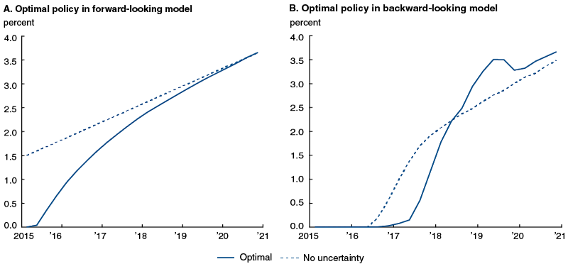
1. Optimal interest rate paths under 2015:Q1 conditions
EFGK study the buffer stock channel in a backward-looking variant of the model discussed above, in which past values of the inflation and output gaps replace their forward-looking counterparts in the Phillips and IS curves. The idea is that output and inflation contain some underlying momentum due to adaptive expectations, inflation indexation, habit persistence by consumers, or costs of adjusting labor or capital inputs. The lagged values of the output and inflation gaps capture this momentum.
Suppose the economy starts with both gaps equal to zero. In order to keep current gaps closed, the central bank will move the nominal interest rate one for one in response to shocks to the natural interest rate.7 As long as the natural rate is positive, the central bank will be able to do this and keep the output and inflation gaps closed. But if the natural rate becomes sufficiently negative, the best the central bank can do is set the policy rate at its ELB and experience negative gaps.
Now suppose the economy starts with output above potential and inflation above target. These lagged gaps put pressure on current output and inflation to remain above their ideal levels. But this also means that the current interest rate would have less stimulative work to do in the event of a negative shock to the natural rate of interest, leaving a smaller chance of running into the ELB. We call this logic the buffer stock channel. Faced with higher odds of a negative natural rate shock tomorrow, it makes sense to loosen policy today to raise current output and inflation; these buffers provide an upward boost to output and inflation tomorrow, lowering the odds of having to lower rates to zero to counter negative natural rate shocks. Of course, this buffer comes with costs—the overshooting of output and inflation targets today and possibly tomorrow—which the central bank needs to weigh against the benefits of the buffer when setting policy. EFGK show formally that an increase in uncertainty over the natural rate tomorrow should be countered with lower policy rates today.
2015:Q1-based simulations
To get a better idea of the implications of uncertainty about the ELB on policy, EFGK simulated both the forward and backward models calibrated to the economic conditions we thought prevailed in the first quarter of 2015—the rate of interest at the ELB, an output gap of 1.5%, inflation 0.7 percentage points below target, and a “neutral” rate of interest of 1.5% (this neutral rate corresponds to the sum of a –0.5% real natural rate and a constant 2% inflation target).8 We assumed everyone in the economy expected the neutral rate to move up to 3.75% in six years but that it was subject to random shocks and, hence, there was uncertainty about its future path.
We calculated the optimal policy interest rate path in both models, and we compared these paths to a naive policy in which the central bank acts as if there will be no further shocks to the economy in the future (even though they see the shocks hitting the economy today and in the past).9 Accordingly, the differences between the two paths show the effects of uncertainty over the natural rate on the optimal policy decision—what we call the risk-management element of policy.10 EFGK provide the details of this exercise.
Figure 1 shows policy paths from the forward-looking model (panel A) and the backward-looking model (panel B) based on 2015:Q1 conditions. These paths are medians from a large number of simulations. The dotted lines give the naive policy and the solid lines the optimal policy. We see that risk-management considerations associated with uncertainty about hitting the ELB meant optimal policy was looser than naive policy. In the forward-looking model, optimal policy called for delaying liftoff by two quarters, and its interest rate path ran 50–150 basis points lower than the naive path for about two years. In the backward-looking model, optimal policy called for delaying liftoff three quarters longer than the naive policy, which, because of the large shortfalls in inflation and output from their goals, already held back rate increases for six quarters. The optimal rate path is below the naive one for about a year before rising more sharply and actually overshooting it later in the simulation.
2017:Q1-based simulations
How have these paths been influenced by changes in the economic environment since we ran these experiments? As of 2017:Q1, it appears that the output gap has essentially closed and that core PCE (personal consumption expenditures) inflation is only about 0.25 percentage points below target. Though smaller than in 2015:Q1, the 2017:Q1 output gap is similar to the two-year-ahead values found in the median simulations in EFGK; i.e., the output gap is in line with what we expected. The inflation rate is about in line with the two-year-ahead level in the forward-looking model and about 0.25 percentage points higher than in the optimal policy simulation from the backward-looking model.
2. Change in neutral rate of interest assumptions
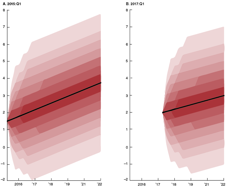
Also, as we noted in the introduction, there is a growing consensus that a slower rate of potential output growth and strong international demand for U.S. assets have lowered the natural rate of interest over the long run. In light of this, we now assume a path for the neutral rate in which the mean slowly rises from 2% today to 3% by 2021. This starting value is close to where EFGK had assumed the median rate would be in 2017:Q1. The terminal value is the median projection for the long-run federal funds rate in the FOMC’s March 2017 SEP.
Figure 2 shows the original and new paths for the neutral rate of interest. The black line is the median expected path for the neutral rate, and the shaded bands show the 10th through 90th deciles of the realized path when we subject the neutral rate to random shocks over time. Despite the increase in the assumed neutral rate since EFGK, the new path runs nearly the same risk of encountering the ELB in the short run. In the medium and long term, the lower terminal point for the neutral rate produces greater odds of hitting the ELB than the path we conditioned our earlier analysis on.
3. Optimal interest rate paths under 2015:Q1 and 2017:Q1 conditions
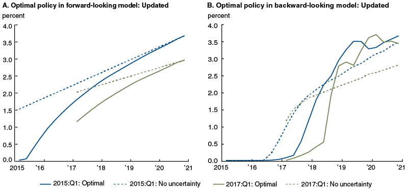
Figure 3 adds the naive and optimal policy paths calculated under these new assumptions (the green lines) to those we calculated in EFGK (the blue lines). Consider first the results for the forward-looking model in panel A. In this model, the naive policy sets the interest rate equal to the neutral rate. As seen, the lower path for the neutral rate and the greater odds of hitting the ELB in the future induce a large policy response today, as optimal policy is 75 basis points below the naive policy. Policy needs to loosen significantly to offset the effects on output and inflation today of the greater odds of hitting the ELB tomorrow. Furthermore, optimal policy in 2017:Q1 is about 50 basis points below the calculation based on 2015:Q1 starting values. In this simple model, the higher chances of hitting the ELB tomorrow more than offset the improved economic conditions over the previous two years. The revision to the path for the neutral rate of interest has a meaningful influence on the policy calculations.
The story is more complicated in the backward-looking model, depicted in figure 3, panel B. Comparing the blue and green dashed lines, we see the improvements in the output gap and inflation rate since 2015:Q1 mean that the naive policy prescribes a higher funds rate than it would have based on our earlier starting assumptions. The same cannot be said for the optimal policy path. The fed funds rate liftoff is delayed until the middle of 2017 under both sets of initial conditions. But, over the next year and a half, the heightened risk of hitting the ELB in the future under 2017:Q1 conditions induces a stronger departure of optimal from naive policy and prescribes a lower fed funds rate path than that based on 2015:Q1 starting values. By mid-2018, the optimal paths are roughly the same, despite the lower path for the neutral rate in the 2017:Q1-based simulations. This reflects the large buffers produced by the additional stimulative policy using 2017:Q1 conditions, which provides large and long-lasting insurance against potential ELB realizations.
The key message from both models is the same: The risk-management consideration, captured in figure 1 as the difference between the solid and dashed lines, is still large today. It is also larger by this time than we expected it to be when we were looking ahead in early 2015.
Conclusion
Updating the calculations of EFGK shows that risk-management considerations associated with the ELB remain important in the current macroeconomic environment. The perception of a lower long-run value for the natural rate of interest is a key factor driving this result. We should emphasize that our conclusions are based on very stylized models, calibrated to match approximately just a few characteristics of the macroeconomic data. Furthermore, they ignore a range of important monetary policy issues, such as unconventional monetary policy, the desire of the central bank to smooth interest rates, financial stability concerns, and the interactions between the central bank’s commitments and private sector expectations. Accordingly, the results are only illustrative. Nevertheless, they do suggest that ELB risks associated with a low long-run value of the natural rate of interest have the potential to influence risk-management considerations for some time.
1 The ELB arises because households and firms can always use cash, which pays zero interest, as a store of value. Some central banks, e.g., the European Central Bank, have been able to set their policy rates to negative values, presumably because it is costly to use cash as a store of value.
2 See Charles Evans, Jonas Fisher, François Gourio, and Spencer Krane, 2015, “Risk management for monetary policy near the zero lower bound,” Brookings Papers on Economic Activity, Spring, pp. 141–219, for reasons why unconventional tools might be imperfect substitutes for conventional interest rate policy.
3 See Jonas D. M. Fisher and Christopher Russo, 2017, “Recent declines in the Fed’s longer-run economic projections,” Chicago Fed Letter, Federal Reserve Bank of Chicago, No. 375, for a discussion of how the SEPs and private sector longer-term forecasts have changed in recent years.
4 The natural rate of interest is the real interest rate that would balance savings and investment over time.
5 For convenience, we assume the ELB is zero in our models.
6 Since gaps are zero if the ELB doesn’t bind and negative if it does, the expected value of the gaps (which averages the possible values of the gaps in both situations weighted by the odds that they occur) must be negative.
7 Technically there is no “natural rate” in the backward-looking model. We use this term loosely to indicate the real interest rate consistent with no shocks to the economy and current and past gaps equal to zero.
8 Potential output—and hence the output gap—and the real natural rate of interest are unobserved. We based our assumptions on common estimates found in early 2015.
9 We assume that policymakers optimize under discretion—i.e., instead of committing to a path or function for the interest rate today forever into the future, they reoptimize policy period by period with the realization of the shocks to the economy. Households and businesses understand this behavior and act accordingly.
10 Note that in the forward-looking model, the naive policy sets the interest rate equal to the natural rate of interest. The naive policy is somewhat different in the backward-looking model, as it may take a number of periods to unwind past shocks to output and inflation gaps.


