Risk Management for Monetary Policy Near the Zero Lower Bound

In a speech to the Peterson Institute I gave last September, I argued that the Federal Open Market Committee (FOMC) would be well served by being especially cautious before raising the fed funds rate off zero. In this paper, Jonas Fisher, Françcois Gourio, Spencer Krane and I develop explicit theoretical and empirical foundations for this argument.

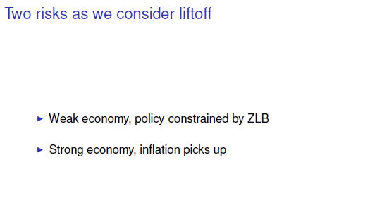
We see two substantial and conflicting risks facing policymakers today. Suppose that the FOMC raises rates, but then discovers that the economy is more reliant on policy accommodation than previously thought — either growth turns weaker or inflation remains stubbornly low. In this situation, the Fed could find itself forced back to the zero lower bound (ZLB). The unconventional tools we have to provide accommodation at the ZLB are useful, but they are imperfect substitutes for changes in the funds rate. And these unconventional tools may be less effective going forward if a premature exit reduces the public’s confidence in the Fed’s commitment to its goals.
 
The other substantial risk is higher inflation. Suppose the FOMC delays raising rates so long that inflation rises much faster than currently projected. Well, the Fed knows how to respond to that — we can raise rates to reel inflation back in. And if the economy is on a solid footing, these rate increases should be manageable. To me, this suggests we should err on the side of less aggressive policy tightening. 

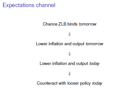
We call the first channel the “expectations channel.” We explore this using the standard workhorse forward-looking New Keynesian model. In that model, when the ZLB binds, both output and inflation are low. So the chance that the ZLB will bind tomorrow translates into lower expected output and inflation tomorrow. And because agents are forward looking, the expected losses tomorrow reduce output and inflation today through negative wealth effects and lower inflationary expectations. In this situation, what should the policymaker do? Our analysis shows that optimal policy under discretion is to loosen policy now.

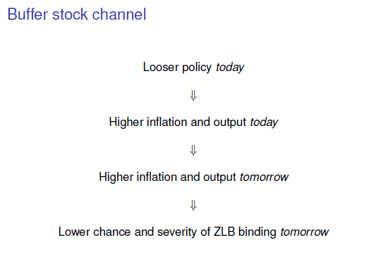
We call the second channel the “buffer stock channel.”

We explore this using an “old-style Keynesian” framework, in which growth and inflation have some inherent underlying momentum due to inertia. This is summarized by the output gap and inflation being functions of their own lagged values. In this setup, the higher output and inflation are today, the higher output and inflation will be tomorrow, reducing in turn the chances that the ZLB will bind tomorrow.

Suppose there is a significant chance a shock tomorrow will push you towards the ZLB. We show that policy should be looser today to build up a buffer of inflation and output so that if that shock does occur, you are less likely to actually hit the ZLB tomorrow. And even if you do get pushed to the ZLB tomorrow, the buffer lowers the costs of doing so.

Naturally, there is a cost from this policy if the shock does not occur and the economy “overheats.” The resulting inflation will have to be brought down. Optimal policy under discretion recognizes these costs and balances them against the benefits that the buffer provides against the ZLB.

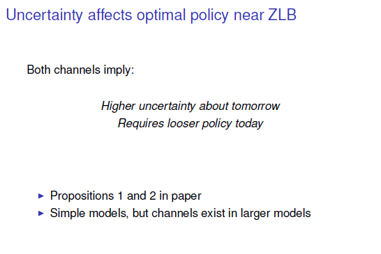
Our theoretical analysis formally develops these two channels.

We have two propositions — one for each model. But they essentially amount to the same thing: As uncertainty rises regarding future shocks that can drive policy to the ZLB, the looser today’s policy should be to guard against those events.

This policy amounts to taking out insurance today against the risk of hitting the ZLB tomorrow. So these propositions certainly fit into a common-sense view of risk management.
 
For analytical convenience and clarity, we present the two channels independently in different simple models. However, both channels operate in standard macro models, such as the state-of-the-art dynamic stochastic general equilibrium (DSGE) models.

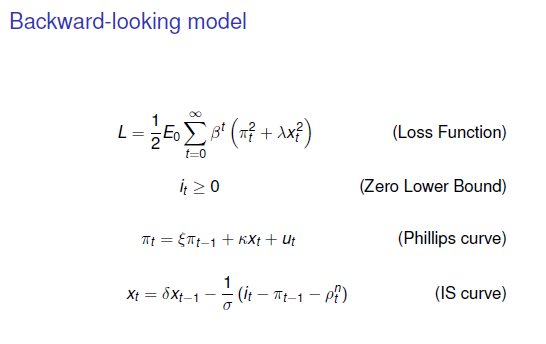
My time is short, so I will briefly illustrate some of what we find using a very standard backward-looking model.

In this model, optimal policy is the interest rate chosen to minimize the usual quadratic loss function of the deviation of inflation from target, π, and the output gap, x. This choice is made subject to being constrained by the ZLB and taking into account private sector behavior, which is governed by the backward-looking Phillips and investment/saving (IS) curves. All of the uncertainty in the model surrounds the cost-push shock denoted by u_t in the Phillips curve and shocks to the equilibrium “natural” real interest rate denoted by ρⁿ in the IS curve.

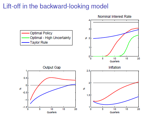
We simulated this model using standard parameter settings from the literature. In period zero, the output gap is –1-1/2 percent, inflation is 1.3 percent (the latest reading for the price index for core personal consumption expenditures, or PCE), and the natural rate of interest is –1/2 percent.

We then assume the real natural rate rises gradually to its long-run level of 1-3/4 percent over the next four years. Uncertainty is modeled as first-order autoregressive, or AR(1), shocks about this natural rate path and in the cost-push term.

With these settings plugged into the model, the optimal policy has the nominal interest rate at the zero lower bound in the first period. The red line in the upper right panel shows the optimal interest rate as we march through time. Obviously both the private sector and the Fed react to shocks as they hit the economy, and there are many possible outcomes. This line is a “baseline scenario,” in which agents make decisions taking into account the model’s uncertainty, but ex post all shocks turn out to be zero. This is akin to plotting an impulse response path.
 
Note that optimal policy delays liftoff from the ZLB for six periods. The resulting output gap is shown by the red line in the lower left panel. The gap falls immediately from –1-1/2 percent at time zero to –1 percent at time one. The output gap eventually overshoots zero, but this is needed to bring inflation — the red line in the lower right panel — back up to target and to maintain a buffer against the ZLB.

For the sake of comparison, we plotted the blue lines, which show what the 1993 Taylor rule would generate. The Taylor rule would immediately set the nominal rate to 2 percent. Output takes four years to return to its potential level, and inflation remains low for a long time.

Finally, the green line in the upper right panel shows what optimal policy looks like if uncertainty increases by 50 percent. Consistent with our theorem, optimal policy in this scenario has liftoff delayed by a further six quarters.

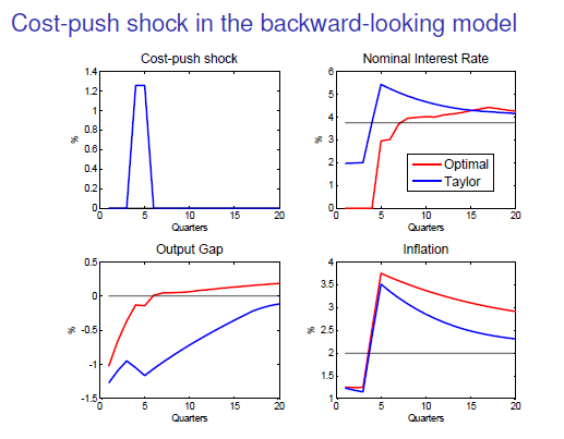
Of course, the baseline scenario is just one possible realization out of many. The next slide considers a scenario that exhibits what many think of as the biggest risk to delaying liftoff — inflation could take off to unacceptably high levels. Here we assume that two large back-to-back cost-push shocks lead to a burst of inflation before what would otherwise be the time for liftoff. These shocks stand in for some unexplained jump in inflation expectations or for other inflationary forces beyond those captured in the model’s simple Phillips curve.

You can see in the upper right panel that both optimal policy and the Taylor rule hike rates aggressively in response to these shocks. Optimal policy clearly does a much better job in closing the output gap than the Taylor rule. And while the Taylor rule does a better job bringing inflation back to target, the inflation path under optimal policy is not radically different. In other words, delaying liftoff does not seem to seriously impair the Fed’s ability to hold inflation in check.

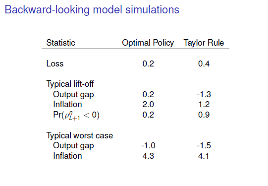
This table summarizes the outcomes from a large number of simulated paths of the natural rate and cost-push shocks using the same set of initial conditions as before. Optimal policy has the smaller loss — about 1/2 of that under the Taylor rule. We find it revealing to look at the economic conditions under which liftoff occurs. In the typical, that is, median, draw, optimal policy lifts off with a small positive output gap and inflation essentially at target. This looks like a “whites of their eyes” inflation-fighting policy.

The optimal policy greatly reduces the odds of hitting the ZLB tomorrow — the probability that the natural rate is negative the quarter after liftoff is only about 20 percent under optimal policy.

These outcomes are very different than under the Taylor rule, which typically lifts off with large negative gaps and 90 percent of the time runs into a negative natural rate immediately after liftoff. 

How well do the policies guard against bad luck? At the bottom, we see the median worst outcomes across simulations. Optimal policy and the Taylor rule are not very different here — worst-case output gaps of 1 percent or so and inflation rates in the range of 4 percent. These results reinforce the point we noted from the previous chart: Optimal policy is able to raise rates enough to choke off inflation scares — and can do so essentially as well as the Taylor rule.

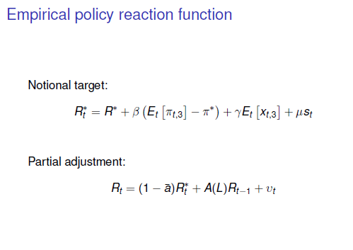
How has risk management entered into actual FOMC policymaking? In our empirical analysis, we study a time span when the funds rate is mostly well above zero. Nevertheless, this history is still worth investigating: If the Fed has practiced risk management away from the ZLB, it seems reasonable for it to take account of the special risks generated by the ZLB in its decision-making calculus today. We study risk management empirically by estimating standard Clarida-Galí-Gertler-style monetary policy reaction functions.
 
Here R-star is a notional target funds rate that depends on the expected difference of inflation from its target and the expected average output gap over the next year. We use the Fed’s Greenbook forecasts for these variables. We then append a variable s_t that proxies for risk-management factors that might influence the policy decision over and above how they might affect the forecast. As is standard, we assume a partial adjustment of the actual funds rate to this notional target.

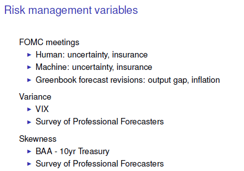
We consider an eclectic mix of risk-management proxies.

The FOMC’s minutes and other Fed communications suggest risk management was often a consideration affecting policy moves. There are numerous references to uncertainties over the outlook; insurance against skewed losses; or preemption of nascent recessionary dynamics.

We summarize this information by coding dummy variables to indicate when we judged uncertainty and insurance considerations shaded policy higher or lower than prescribed by the forecast alone.

We also let the computer take a shot at this, by having it count sentences in the minutes that mention “uncertainty” and “insurance.” Other proxies include revisions to Greenbook forecasts for gross domestic product (GDP) and inflation — large forecast revisions may signal asymmetric weights on outcomes in the direction of the shock and the FOMC may have wanted to insure against these outcomes. We also consider variables that summarize variance and skewness in private sector forecasts, including those derived from financial markets and those derived from the Philadelphia Fed’s Survey of Professional Forecasters (SPF).

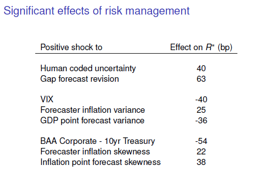
Here are the variables we found statistically significant at the 5 percent level. When the human-coded uncertainty dummy turns on up or down, the notional target funds rate changes by 40 basis points. All other numbers are the basis point responses to the notional target associated with a one standard deviation increase in a variable. Overall, we find what our historical narrative analysis also suggests: Before it was constrained by the ZLB, the FOMC seems to have incorporated risk-management considerations into its policy decisions.

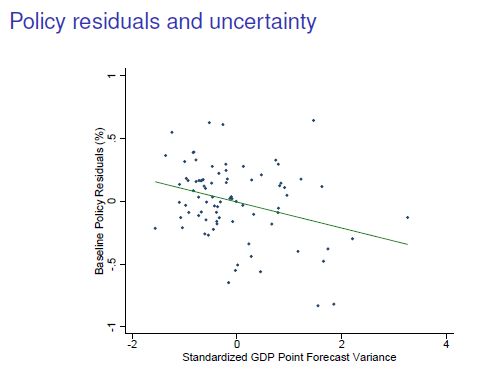
This chart shows how one of our proxies — the variance across the GDP point forecasts made by the SPF panelists — lines up with the residuals from the policy reaction function that excludes a risk-management proxy. We see a clear negative correlation, suggesting the Committee shaded down the funds rate during times when the private sector — and, presumably, the Fed — had heightened uncertainty over the outlook for growth.

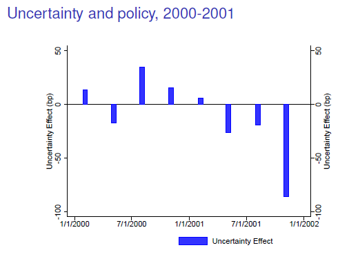
It’s useful to look more closely at the 2000–01 period.

The bars in this figure show the effect on the notional funds rate of the GDP point forecast variance shown in the previous figure. The bars are quarterly because this is the frequency of the SPF.

By the middle of 2000, the economy appeared to be slowing, in part because of monetary tightening in 1999 and early 2000. The level of our proxy for uncertainty usually was below average then. But as we moved through 2001, the economy slowed more, and uncertainty grew about whether we were slipping into recession — this shows up here as negative effects of the uncertainty variable.

Then, the tragic events of September 11th hit, which created huge uncertainty and downside risks to the economic outlook. We see this in the spike in the SPF uncertainty variable in November — the last bar — that would point to a nearly 100 basis point drop in the funds rate.

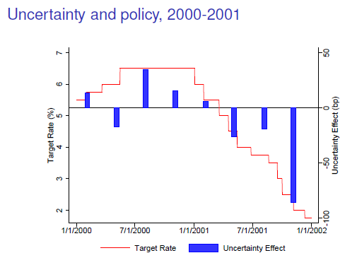
The red line plots the actual path for the funds rate against these uncertainty effects. We can see that the Fed began to undo its tightening cycle in mid-2000, and cut rates a good deal further in mid-2001as uncertainty rose. We then see that the large spike in uncertainty at the end of the year is correlated with a big drop in the funds rate.

Of course, there is much more to be said about risk management during this period. The 2000 pause in rate increases occurred despite forecasts of very low unemployment and rising inflation, in part, as the minutes tell us, because the Committee was uncertain over the degree to which its previous tightening might further affect the economy.

The aggressive rate cuts in early 2001 encompassed other rationales; notably, the January 30–31, 2001, minutes stated the Committee was front-loading easing to “help guard against cumulative weakness” — perhaps a reference to policy insurance against outcomes skewed to the downside.

The post-9-11 cuts had this reasoning as well. In addition, as evidenced in the November 6, 2011, minutes, the Committee noted its concern that recessionary dynamics could, and I quote, “be difficult to counter with the current federal funds rate already quite low.” Accordingly, the large policy moves could also have reflected insurance against the future possibility of running into the ZLB — precisely the policy scenario our theory addresses.

So, to conclude, we think our theoretical and empirical analysis support one of my favorite quotes from one of our discussants: