

Do people adjust how much they want to work when the central bank’s monetary policy stance shifts? More specifically, does an interest rate hike induce individuals to work more or fewer hours? And does this effect differ across households with different levels of income (or earnings)? In this article, we discuss our recent research that explores these and related questions. One notable finding is that employed individuals at the bottom of the income distribution want to work more when monetary policy tightens.
Conventional wisdom about the transmission of monetary policy suggests that households would reduce how much they want to work—i.e., their desired labor supply—in response to an interest rate hike. In particular, the lower wage rates induced by contractionary monetary policy have two effects on households’ labor supply decisions. On the one hand, when monetary policy tightens, there’s a substitution effect that reduces how much households would like to work: Given the relatively lower return on their labor, they prefer to substitute away from the time they devote to work to other activities. On the other hand, when monetary policy tightens, there’s also an income effect that increases how much households would like to work: Because their purchasing power will be lowered by the rate hike, households want to devote more of their time to work in order to raise their incomes. With that said, it is often thought that income effects on the labor supply associated with monetary policy shocks are small; because these effects are so short-lived, they do not have large effects on lifetime income.
In Cantore et al. (2022), we study the effect of monetary policy on labor supply decisions at a more granular and disaggregated level using survey data on U.S. households. Our analysis finds that responses differ substantially across different income (or earnings) groups. In particular, we find that while aggregate hours worked and labor earnings decline following a monetary policy tightening, employed individuals at the bottom of the income distribution actually work more hours; i.e., individuals with jobs at the bottom of the income distribution display countercyclical behavior—or behavior that is negatively correlated with business cycle fluctuations in gross domestic product (GDP).
In this Chicago Fed Letter, we go over the data we used and the empirical model we developed for Cantore et al. (2022). Moreover, we present our model’s results for how various macroeconomic and disaggregated labor market indicators behave following a monetary policy tightening. These results show how differently employed people at the bottom of the income distribution respond to a rate hike, compared with the total population or with people who have higher incomes.
The data and the empirical model
In Cantore et al. (2022), we consider two sources of individual- and household-level data: the Current Population Survey (CPS) and the Consumer Expenditure Survey (CEX). The former survey is the primary source of labor force statistics for the population of the United States; the latter survey collects information on expenditure and income to study the buying habits of U.S. consumers. Both surveys contain useful information about households’ labor supply decisions and their income or earnings distribution. The CPS is conducted at a monthly frequency on a sample of about 60,000 U.S. households; it contains detailed information about the demographic characteristics of the household, labor market attitudes, and labor earnings. Available at a quarterly frequency,1 the CEX is based on a smaller sample than the CPS;2 however, compared with CPS data, CEX data contain more detailed information about households' income sources. Therefore, from the CPS we can use individual-level data on hours worked and hourly wages, but we can only sort individuals based on their labor earnings (and not gross income). And from the CEX we can use household-level data on labor income and hours worked, yet we can only sort households based on their gross income. This means that the results from the two surveys are complementary, but not directly comparable.3
To estimate the impact of monetary policy shocks on the labor supply decisions of different segments of the population by income or earnings, we use a factor-augmented vector autoregressive (FAVAR) model. Our FAVAR model combines the household- and individual-level data (from the CEX and CPS) on hours worked at different percentiles of the income or earnings distribution with the information contained in a large set of aggregate time series covering real economic activity, employment, inflation, money, credit, credit premiums,4 and asset prices.5 According to our model in Cantore et al. (2022), observed outcomes in this rich data set are the results of a variety of supply and demand shocks hitting the U.S. economy at different times. To isolate monetary policy shocks, we relate the empirical model’s innovations (i.e., the unpredictable component of the variables in the data set) to an observed proxy for monetary policy surprise built using intraday data on three-months-ahead federal funds futures. Changes in this instrument during a tight window around meetings of the Federal Open Market Committee likely reflect unexpected changes in monetary policy. The dynamic transmission of the monetary policy surprise to aggregate and household-level variables is computed with our FAVAR model.
Responses of aggregate and disaggregated variables
Figure 1 shows the responses of some key aggregate variables to a contractionary monetary policy shock corresponding to a 1% increase in the one-year Treasury constant maturity rate; in particular, the blue line in each panel of the figure displays the point estimate (median) response and the dark and light gray areas indicate the 68% and 90% Bayesian confidence sets, respectively (the time unit on the horizontal axis is a quarter). In the six panels of figure 1, we present the responses of the one-year interest rate, real gross domestic product, the Consumer Price Index (CPI), the Standard and Poor’s 500 stock market index (S&P 500),6 the unemployment rate, and the hours worked for all employed individuals in the business sector.
1. Responses of macroeconomic variables after a monetary policy tightening
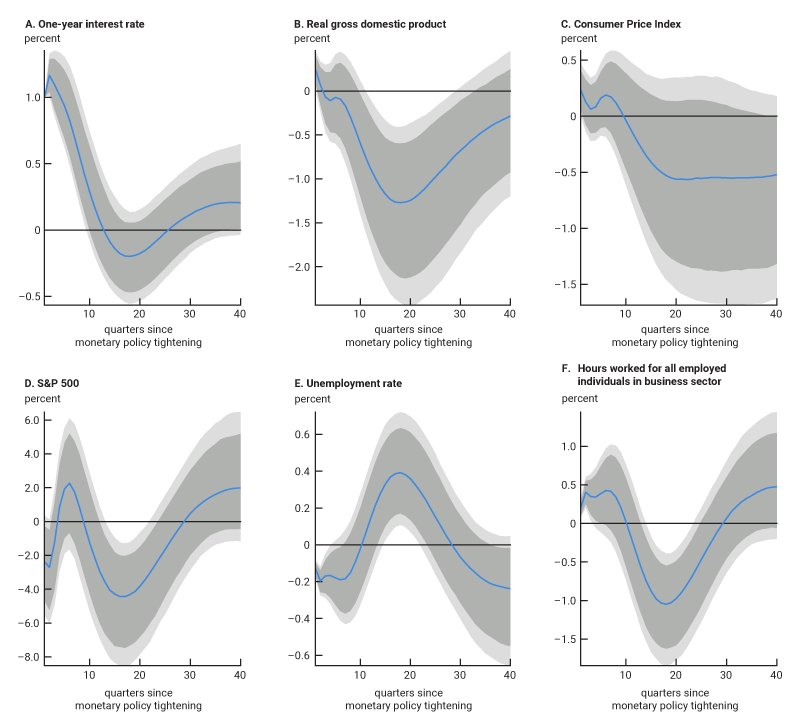
Source: Cantore et al. (2022).
The peak decline in real GDP reaches 1.3% below its long-run trend four years (16 quarters) after the monetary policy tightening. The fall in real GDP coincides with a rise in the unemployment rate of 0.4% and a decline in total hours worked of 1% (both relative to their respective long-run trends) at about the same time. The S&P 500 reacts negatively, and the CPI sluggishly declines. Several other economy-wide variables display interesting dynamics after a contractionary monetary policy shock (not shown here). In particular, the main components of aggregate demand—i.e., consumption and investment—and standard measures of industrial production (both aggregate and sectoral) all decline. Like the CPI, producer and other consumer price indexes contract. A number of labor market indicators deteriorate after the rate hike: Employment in the aggregate and for various specific industries falls, and real wages and compensation decline. Standard monetary aggregates drop, and liquidity becomes scarcer. Household financing costs rise. Corporate credit costs (e.g., the U.S. excess bond premium) rise over the short and medium terms. Overall, these estimated dynamics are consistent with the typical narrative following a monetary policy tightening.
Figure 2 shows the responses of hours worked for households in different income or earnings groups. In particular, panel A of figure 2 displays the response of hours worked for employed households in the third quintile of the CEX income distribution (the middle fifth of the sample), and panel B displays the response of hours worked for employed households in the first quintile (the lowest fifth). In addition, panel C shows the response of hours worked for employed individuals in the first decile of the CPS earnings distribution (the lowest tenth of the sample), and panel D displays the response of the unemployment rate7 for those in the first decile of the CPS earnings distribution. The dynamic response of hours worked by households in the third quintile of the income distribution (which includes the median-income households) is qualitatively similar to the dynamic profiles of aggregate quantities, e.g., real GDP (see figure 1, panel B); as shown in figure 2, panel A, it slowly declines, reaching its trough four years (16 quarters) after the monetary policy shock. In contrast, the response of hours worked by households or individuals below a certain income or earnings threshold (the first quintile of the CEX or first decile of the CPS) is countercyclical. In particular, households in the first quintile of the CEX income distribution increase their labor supply rapidly a few quarters after the negative demand shock induced by contractionary monetary policy (see panel B of figure 2). Moreover, this effect tends to be persistent and the increase in labor supply is still significant two years after the shock. The individual responses obtained using the CPS data are qualitatively similar to the findings based on the CEX data (see panel C of figure 2); the magnitudes are different and the uncertainty surrounding these estimates is larger. That said, from panels B and C, it’s clear that a significant share of the U.S. population with low incomes or earnings tends to increase its labor supply after a monetary policy tightening.
2. Responses of hours worked and the unemployment rate by income or earnings group after a monetary policy tightening
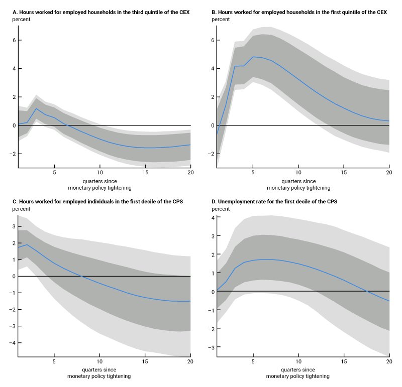
Source: Cantore et al. (2022).
One caveat of this analysis is that the hours worked for different income or earnings groups are not constructed using the same households or individuals over time and there might be composition effects of people switching jobs and/or going in and out of the labor force in between survey data collection. In particular, the strength of the income effect on the labor supply could be the result of two mechanisms: more people at the bottom of the income or earnings distribution entering the labor market (extensive margin) and employed people working longer (intensive margin). Because the unemployment rate for individuals with low earnings does not decline after a monetary policy shock (see panel D of figure 2), we can rule out large movements in the extensive margin. Hence, after a negative demand shock induced by a monetary policy tightening, individuals with low incomes or earnings who remain in the labor market tend to work longer hours. Moreover, the other important piece of evidence consistent across surveys is that labor market outcomes are more sensitive to monetary policy shocks at the lower end of the income or earnings distribution.
Conclusion
We have documented here how households across the income (or earnings) distribution differ in terms of how many more or fewer hours they would like to work in response to a monetary policy shock. While aggregate work hours decline after a monetary policy tightening, the actual labor supplied by households with low incomes, conditional on keeping their jobs, increases. This increase in labor supply is not typical of the narrative following an interest rate hike.
There are several possible explanations for our finding of strong income effects on the labor supply decisions of households with low incomes. As the recession induced by contractionary monetary policy increases the probability of becoming unemployed, households with limited income sources face larger risks; thus, to insure themselves against possible future income losses, members of such households might want to work more hours while they’re still employed. An alternative plausible explanation is liquidity constraints: Individuals who are close to their borrowing limits might desire to work more hours to meet their debt obligations when interest rates rise. Finally, another reasonable explanation is that there’s only so much spending that households with low incomes can cut back on; given that the consumption bundle of such households typically contains a large share of necessities, their ability to reduce consumption might be limited when their hourly labor earnings decline. Eventually these households’ hours worked would need to increase to meet their consumption needs. It is very difficult to isolate the channel responsible for our empirical finding. However, all of these mechanisms suggest that when lacking buffer savings or nonlabor income sources, those with low incomes have less room to maneuver in tough economic times; therefore, they are more inclined to adjust how much they work in response to monetary policy shocks, such as an unexpected interest rate hike.
Notes
1 CEX data are collected by the U.S. Census Bureau for the U.S. Bureau of Labor Statistics in two surveys: a quarterly interview survey, which gathers data about major and/or recurring items, and the more frequently conducted diary survey, which gathers information on more minor or frequently purchased items. Combined, the data from both the interview and diary surveys cover the complete range of consumers’ expenditures; this complete set is only available at a quarterly frequency. See also note 2. Further details on CEX data collection are available online.
2 The CEX is a monthly rotating panel, where each household is interviewed once per quarter, for at most five consecutive quarters. Income and hours worked data are collected from interviews conducted in the second and fifth quarters, and financial data are only collected in the fifth (final) interview. The reference period for income flows covers the 12 months before the interview. To construct the quarterly variables for our research, we retain the consumer units (CUs) from the second interview or the fifth interview in each year of the sample when income data are updated. CUs are then assigned to each quarter of the year by their date of interview (see Cloyne and Surico, 2017), and then they are sorted into bins by gross income.
3 We apply a filter to both the CPS and CEX data for our research. In particular, we drop respondents who are in the top and bottom one percentile of the earnings distribution (in the CPS) or income distribution (in the CEX), as well as respondents who are younger than 18 or older than 66. Moreover, at each point in time (i.e., in the month for the CPS or the quarter for the CEX), we construct different earnings and income percentile groups (deciles and quintiles). For more details on our data constructions, household demographics, and income characteristics, see Cantore et al. (2022).
4 By credit premiums, we are referring to, for instance, the difference between corporate and government bond interest rates.
5 The macroeconomic and financial time series data are obtained from the St. Louis Fed’s FRED-QD and FRED-MD databases, available online. The quarterly data that we use from FRED-QD contain 238 time series and cover the period from 1984:Q1 through 2018:Q4. Accounting for the same broad categories as the quarterly data, the monthly data that we use from FRED-MD contain 137 time series; however, the monthly data cover a relatively shorter period—from January 1994 (when the first observation of hours worked constructed in the CPS was recorded) through December 2019.
6 Details on the S&P 500 are available online.
7 To construct unemployment rates at various percentiles of the CPS earnings distribution, we use Mincer-type regressions to impute hourly earnings for those individuals who are unemployed. In particular, we regress earnings on the level of education, a measure of experience (age minus years of schooling minus six), and individual characteristics (including race, gender, and industry of occupation). The fitted values from this regression are used to obtain imputed earnings for unemployed individuals. The coefficients of the regression are shocked and used to produce predicted values. These are assigned to unemployed individuals, using predicted mean matching. We produce five replicates, with the final imputed data taken to be the mean across these replicates. We then compute the distribution of earnings (including those unemployed with imputed income); and for each percentile, we compute the fraction of unemployed people.


