

Introduction and summary
In many countries, employers are forced to make large severance payments to workers when their employment is terminated for reasons other than worker misconduct.1 Actually, it is not uncommon for severance payments to exceed 20 days of pay per year worked, with a cap of one year of wages (for example, in Argentina, Italy, and Spain). In addition, employers often face substantial legal costs when they terminate their workers. Economic theory indicates that these firing costs have large effects on the hiring and firing decisions of firms. Not surprisingly, in an effort to economize their immediate costs, firms respond to the firing costs by reducing their firing rates. However, because they are afraid of the costs that they will have to face in the future, firms also respond by reducing their hiring rates. The net effects on their employment levels depend on whether the decrease in firing rates exceeds the decrease in hiring rates. While their effects on average employment are ambiguous, firing costs generate a clear misallocation of labor across firms. The reason is that firms that receive positive shocks do not expand as much as they should and firms that receive negative shocks do not contract as much as they should. Perhaps because of this misallocation of resources across firms, governments have introduced legislation attempting to improve the efficiency of their countries’ labor markets. One common way that governments have done this is through the introduction of temporary employment contracts of fixed lengths. These temporary contracts effectively provide a period of time during which workers can be fired at no costs. If a temporary worker is retained after their temporary contract ends, they become a permanent worker subject to regular firing costs. The purpose of this article is to provide a quantitative assessment of temporary contracts. In particular, we are interested in determining how effectively temporary contracts of observed length bring the economy close to laissez-faire outcomes (that is, to the economic outcomes that would be obtained under zero firing costs to firms).
In order to do this, we consider the equilibrium search model of Alvarez and Veracierto (2012), which is an undirected search version of the Lucas and Prescott (1974) model with an out-of-the-labor-force state. The economy comprises a continuum of islands and a home sector. Each of the islands has a unit interval of identical firms that produce output with a decreasing returns to scale production function that uses labor as its sole input. Islands are subject to idiosyncratic productivity shocks that follow a Markov process over time. Agents value consumption and home production, and start every period of time either at home or at one of the production islands in the economy.2 If an agent starts a period of time at home, they can choose either to stay at home during the current period or to search. Staying at home allows them to enjoy home production during the current period, but makes them start the following period at home again. Searching precludes the agent from obtaining any home production during the current period, but allows them to randomly arrive at one of the islands at the beginning of the following period (search is undirected). If an agent starts a period of time at one of the islands, they can choose either to stay on the island (and work), to randomly search for a new island, or to go home. Only going home and staying there provides home production to the agent. The amount of home production obtained by staying at home is the same for all individuals.
In this framework we introduce a government policy that taxes firms for reducing their employment of workers with J or more periods of tenure on the island.3 The firing tax on these permanent workers is equal to τ. However, firms do not face any firing tax for reducing their employment of workers with tenure of less than J periods. All the firing taxes collected by the government are rebated as lump-sum transfers to the representative household. The assumption that firing taxes apply to the worker’s tenure on the island (and not to the worker’s tenure in a firm) allows us to specify a standard competitive equilibrium.4 In particular, we assume that there are spot labor markets for each tenure level (thus, potentially, workers of different tenure have different wage rates). Given their previous-period employment of permanent workers, firms maximize the present discounted value of their profits (which are given by output net of wages and any firing taxes incurred). Because we assume that workers are fully insured, they seek to maximize the present expected discounted values of wages and home production.
We use our model to explore to what extent fixed-term contracts of different lengths add flexibility to the labor market.5 Notice that introducing fixed-term contracts of sufficiently large J is equivalent to eliminating all the firing taxes (since workers never gain permanent status). Thus, we address the question of how much labor market flexibility gets generated by computing how much of the gap between the firing-tax case (J = 1 and $\unicode{x03C4} >0$) and the laissez-faire case (either $J=\text{ }\unicode{x221E} $ or $\unicode{x03C4} =\text{ }0$) is closed when fixed-term contracts of empirically reasonable length are introduced. To this end, we consider the case of Spain in the mid-1980s—which introduced long temporary contracts in a labor market characterized by large firing costs. Calibrating the model to a stylized version of that economy, we find that temporary contracts of three years’ duration (roughly the length of the contracts introduced in Spain) close about half of the welfare gap between the firing-tax and the laissez-faire cases.
There is a long theoretical literature analyzing the quantitative effects of temporary contracts in structural models. An early contribution to this literature is Cabrales and Hopenhayn (1997)—who find that the introduction of temporary contracts has large effects on turnover rates in a partial equilibrium dynamic labor demand model that abstracts from unemployment. Interestingly, they find that there is a large increase in the firing rate of workers with tenure equal to the length of the temporary contracts introduced. However, despite the large turnover effects, they find moderate effects on employment. Bentolila and Saint-Paul (1992) and Aguirregabiria and Alonso-Borrego (2014) also analyze partial equilibrium models that abstract from unemployment, obtaining similar results. Veracierto (2007) introduces unemployment into a small open model economy, but in order to analyze short-run dynamics, he assumes a linear production function that leads to equilibrium wages being independent of the aggregate state of the economy and constant across tenure levels; in terms of steady-state employment, he finds that temporary contracts of six months’ duration have small positive effects. Blanchard and Landier (2002) and Cahuc and Postel-Vinay (2002) also introduce unemployment into their models, but they consider versions of the Mortensen–Pissarides matching model; they find that introducing temporary contracts increases job turnover but can reduce aggregate employment. Güell and Rodríguez Mora (2010) consider a Shapiro–Stiglitz model of efficiency wages and find that when there is a minimum wage, introducing temporary contracts can reduce employment. With this Economic Perspectives article, we contribute to this literature by evaluating the effects of temporary contracts in a Lucas–Prescott islands economy with undirected search. While the theory for this framework has already been provided in Alvarez and Veracierto (2012), the contribution of this article is to provide a quantitative analysis.
In the next section, we describe our model economy. After this, we describe the model economy’s competitive equilibrium—which is flexible enough to capture key features of the Spanish economy both before and after its 1984 labor market reform. Then, we discuss the details of our computational experiments—including the calibration of the model to match Spain’s economy prior to its 1984 reform—and the effects of introducing temporary contracts to that economy. Finally, we provide our concluding remarks.
The economy
There is a single consumption good in the economy that is produced in a unit measure of islands. The production function of each island is given by
\[{{y}_{t}}={{z}_{t}}n_{t}^{\unicode{x03B1} },\]
where \({{z}_{t}}\) is an idiosyncratic productivity shock, \({{n}_{t}}\) is employment, and \(0 \lt \unicode{x03B1} \lt 1\). The productivity shock \({{z}_{t}}\) follows a finite Markov process with transition matrix Q.
The economy is populated by a unit measure of agents. These agents start every period of time located either on one of the islands or at home (see note 2). If an agent starts a period of time on one of the islands, they can choose either to stay or to leave. If they stay, they work on the island during the current period and start the following period located at the same island. If they leave, they have two alternatives available to them: perform home production or search for a new island. If they perform home production, they produce ω units of the home good during the current period and start the following period at home. If they search during the current period, they do not produce but arrive randomly at one of the islands at the beginning of the following period. We assume that search is undirected, so the probability of arriving at an island of any given type is given by the fraction of islands of that type in the economy.6 The agents who start a period of time located at home have the same alternatives available to them as those available to the agents who leave the islands where they were initially located. We denote by \({{L}_{t}}\) the total number of agents who perform home production at time t, by \({{U}_{t}}\) the total number of agents who search at time t, and by \({{N}_{t}}=\text{ }1-\text{ }{{L}_{t}}-\text{ }{{U}_{t}}\) the total number of agents who are employed at time t. We refer to the sum \({{L}_{t}}+{{U}_{t}}\) as the total number of agents who are nonemployed (that is, unemployed or out of the labor force) and to the ratio \({{U}_{t}}_{\ }/\left( 1-{{L}_{t}} \right)\) as the unemployment rate.7
All agents have identical preferences given by
\[{{E}_{0}}\sum\limits_{t=0}^{\unicode{x221E} }{{{\unicode{x03B2} }^{t}}\left[ \frac{c_{t}^{1-\unicode{x03B3} }-1}{1-\unicode{x03B3} }+{{h}_{t}} \right]}\,,\]
where ${{c}_{t}}$ is consumption, ${{h}_{t}}$ is home production, $0\lt\unicode{x03B2} \lt1$ is the discount factor, and $\unicode{x03B3} \ge 0$ is the intertemporal substitution parameter. We assume that there is a unit measure of households, each constituted by a unit interval of agents, and that agents can obtain full consumption insurance within their households.8 The preferences of the representative household are then given by
\[\sum\limits_{t=0}^{\unicode{x221E} }{{{\unicode{x03B2} }^{t}}\left[ \frac{c_{t}^{1-\unicode{x03B3} }-1}{1-\unicode{x03B3} }+\unicode{x03C9} {{L}_{t}} \right]}.\]
Competitive equilibrium
In this section we describe a recursive competitive equilibrium with firing taxes and temporary contracts. Since this competitive equilibrium has been described in detail in Alvarez and Veracierto (2012), only its main ingredients are sketched here.
The state of an island is given by a pair (T, z), where $T=\text{}\left({{T}_{0}},{{T}_{1}},\text{ }...,{{T}_{J}} \right)$ is a vector describing the number of workers across tenure levels present on the island at the beginning of the period and where z is the idiosyncratic productivity shock. While ${{T}_{j}}$ for j = 0, ..., J − 1 represents the number of workers with tenure j, we find it convenient to include in ${{T}_{J}}$ all workers with tenure greater than J − 1. We refer to ${{T}_{J}}$ as the total number of permanent workers, to ${{T}_{0}}$ as the new arrivals, and to ${{\sum }_{j=1,\,...,\,J-1}}{{T}_{j}}$ as the total number of temporary workers. The government imposes on the firms a firing tax $\unicode{x03C4} $ per unit reduction in their employment of permanent workers. However, reducing the employment of temporary workers entails no firing taxes. All firing taxes collected across all the islands in the economy are rebated as lump-sum transfers to the representative household.
In each island there are J + 1 spot labor markets, one for each tenure level j = 0, ..., J. As a consequence, current wages ${{w}_{j}}\left( T,z \right)$ are indexed by the tenure level and the state of the island. In solving their individual problems, both agents and firms not only take the equilibrium functions ${{w}_{j}}\left( T,z \right)$ as given, but also the equilibrium law of motion for the endogenous state of the island ${T}'=A\left( T,z \right)$. This law of motion is needed to forecast future wages on the island.
Because workers are fully insured within their households, they seek to maximize their expected discounted values of wages and home production. In particular, the problem for a worker with tenure j on an island of state (T, z) is to decide whether to become nonemployed or to stay and work. Becoming nonemployed entails a value given by $\unicode{x03B8} $ (to be determined in equilibrium). By staying, the worker receives a wage rate ${{w}_{j}}$ during the current period and gains tenure min {j + 1, J} for the following period. We denote the value function for a j-tenure worker on a (T, z)-island as ${{W}_{j}}\left( T,z \right)$. This value function must solve
\[{{W}_{j}}\left( T,\,z \right)=\max \left\{ \unicode{x03B8} ,\,\,{{w}_{j}}\left( T,\,z \right)+\unicode{x03B2} \sum\limits_{{{z}'}}{{{W}_{\min \left\{ j+1,\,J \right\}}}\left( A\left( T,\,z \right),\,\,{z}' \right)}\,Q\left( z,\,{z}' \right) \right\}\]
for all (T, z) and j = 0, ..., J.
The problem of the representative firm on an island of type (T, z) is simply to maximize the expected present discounted value of its profits—that is, of output net of total wage payments and firing costs. The problem of a firm that employed p permanent workers during the previous period and is on an island of type (T, z) is described by the following Bellman equation:
\[B\left( p;\,T,\,z \right)=\underset{\left\{ {{n}_{j}}\ge 0 \right\}_{j=0}^{J}}{\mathop{\max }}\,\left\{ z{{\left( \sum\limits_{j=0}^{J}{{{n}_{j}}} \right)}^{\unicode{x03B1} }}-\sum\limits_{i=0}^{J}{{{w}_{j}}\left( T,\,z \right){{n}_{j}}-\unicode{x03C4} \,\max \left\{ p-{{n}_{J}},\,\,0 \right\}\,+\,\unicode{x03B2} \sum\limits_{{{z}'}}{B}\left( {{n}_{J}}+{{n}_{J-1}};\,A\left( T,\,z \right),{z}' \right)\,\,Q\left( z,\,\,{z}' \right)} \right\},\]
where B is the value function of the firm. Observe that ${{n}_{J-1}}$ is the employment of workers that in the previous period were at the end of their temporary contracts. When these workers are employed during the current period, they become permanent workers and must be added to ${{n}_{J}}$ for determining the previous-period employment of permanent workers that the firm will have at the beginning of the following period.
At a steady-state equilibrium, the following seven conditions must hold: 1) the employment levels ${{n}_{j}}\left( {{T}_{J}};T,z \right)$ that the representative firm on an island of type (T, z) chooses must generate the law of motion A (T, z) that agents and firms take as given (observe that because of the undirected search assumption, ${{T}_{0}}$ is always equal to the total number of agents who search U), 2) the employment levels ${{n}_{j}}\left( {{T}_{J}};T,z \right)$ must be willingly supplied by the workers with tenure j at an island of type (T, z), 3) the invariant distribution of islands across states (T, z) must be generated by the law of motion A (T, z) and the Markov process that the idiosyncratic productivity shock z follows, 4) the total number of employed agents across all islands in the economy (or total employment) plus the total number of searchers U plus the total number of agents doing home production L must equal one (the total population in the economy), 5) the value of nonemployment $\unicode{x03B8} $ is equal to the expected discounted value of randomly drawing ${{W}_{0}}\left( T,z \right)$ under the invariant distribution of islands (observe that ${{W}_{0}}\left( T,z \right)$ is the value that a newly arrived worker obtains at an island of type (T, z)), 6) the value of nonemployment satisfies that $\unicode{x03B8} =\text{ }{{c}^{\unicode{x03B3} }}\unicode{x03C9} +\text{ }\unicode{x03B2} \unicode{x03B8} $ (that is, the value of becoming nonemployed is equal to the value of doing home production during the current period plus the discounted value of being nonemployed during the following period), and 7) the total output obtained across all production islands in the economy equals the consumption level c enjoyed by the representative household.
In Alvarez and Veracierto (2012), we show that at a steady-state equilibrium there are three levels of wages: one wage level $\bar{w}\text{ }\left( T,\text{ }z \right)$ common to all temporary workers with tenure j = 0, ..., J – 2; another wage rate for the workers that are about to become permanent (that is, j = J − 1); and another wage rate for permanent workers (that is, j = J ). Moreover,
$1)\,\bar{w}\left( T,\,z \right)=z\unicode{x03B1} {{\left( \sum\limits_{j=0}^{J}{{{n}_{j}}\left( {{T}_{J}};\,T,\,z \right)} \right)}^{\unicode{x03B1} -1}},$
$2)\,{{w}_{J-1}}\left( T,\,z \right)\le \min \left\{ \bar{w}\left( T,\,z \right),\,\,{{w}_{J}}\left( T,\,z \right) \right\},$
$3)\,\bar{w}\left( T,\,z \right)\lt{{w}_{J}}\left( T,\,z \right),\,\,\text{if}\,{{n}_{J}}\left( {{T}_{J}};\,T,\,z \right)\lt{{T}_{J}}.$
The intuition for why the wage rate of temporary workers with tenure less than J – 1 is equal to the marginal productivity of labor (equation 1) is that these workers are still far from becoming permanent workers subject to firing taxes and, therefore, firms treat them as being fully flexible. The intuition for why the wages of temporary workers with tenure J − 1 are the lowest (equation 2) is that firms need to be compensated for hiring them because doing so will make the firms subject to firing costs during the next period. The intuition for why the wages of permanent workers are the highest when the representative firm fires some of these workers (equation 3) is that in this case, the marginal value of not firing the last worker is given by the marginal productivity of the worker plus the firing taxes saved.9
Observe that because islands are indexed by the vector T, the curse of dimensionality seems to preclude any possibility of computing equilibriums for values of J significantly larger than 2. However, in Alvarez and Veracierto (2012), we show that independent from the value of J, the endogenous state of an island can always be summarized by only two values: the total number of temporary workers and the total number of permanent workers. The undirected search assumption, under which every island receives U new arrivals every period, is crucial for delivering this simplified representation of the state space and, therefore, for being able to compute equilibriums under moderate values of J.
Computational experiments
In this section we evaluate to what extent the introduction of temporary contracts adds flexibility to the labor market. To this end, we consider as a benchmark the case where J = 1 and $\unicode{x03C4} >0$ and calibrate it to an economy with high separation taxes and no temporary contracts—similar to Spain’s pre-1984 economy.10 Once the benchmark economy, which we refer to as the firing-tax case, is parameterized, we compute competitive equilibriums under temporary employment contracts of different lengths (that is, with different values of J) and evaluate their effects.
For the purposes of comparison, we also compute the equilibrium allocation under zero separation taxes, which we refer to as the laissez-faire case. This is an interesting case to consider because the equilibrium allocation with temporary employment contracts of long duration coincides with the equilibrium allocation under laissez faire. The reason is quite simple: With a large enough J, firms can perfectly replicate their laissez-faire employment levels by using only temporary workers. Given this property, we address the question of how much flexibility the temporary contracts generate by computing what fraction of the gap between the firing-tax and laissez-faire cases is closed when temporary contracts of different lengths J are introduced.
We note that in the laissez-faire case, which is obtained by setting either $J=\text{ }\unicode{x221E} $ or $\unicode{x03C4} =\text{ }0$, the tenure levels of the different workers become immaterial. This implies that while total employment is uniquely determined, the hiring and firing rates across the different tenure levels are undetermined. Despite this, we choose to focus on the employment adjustments obtained as the limit when $\unicode{x03C4} \to 0$ (or equivalently, when $\unicode{x03C4} $ is arbitrarily small). This is useful because it helps emphasize the types of adjustments that temporary contracts lead to even in the case in which they are totally unimportant.11
In the rest of this section, we present the empirical observations from mid-1980s Spain that motivate the computational experiments we conduct; show how we calibrated the model to the pre-1984 Spanish economy; and report the results of the exercises.
Some empirical background
Since the introduction of fixed-term contracts during the 1980s, the fraction of workers hired under this modality had expanded steadily in European Union countries, reaching more than 17 percent by 2000 (Buddelmeyer, Mourre, and Ward-Warmedinger, 2004, figure 3.1, p. 21). However, there are large cross-country differences in the scope and duration of fixed-term contracts. For instance, some countries restrict these contracts to certain occupations and types of workers, while others give them broad applicability. In what follows we focus on the case of Spain, because in 1984 Spain substantially liberalized the applicability of temporary contracts at a time when the country had one of the highest employment protection levels in Europe (see Cabrales and Hopenhayn, 1997, and Heckman and Pagés, 2000). From 1984 to 1991, the fraction of workers with fixed-term contracts in Spain went from 11 percent to more than 30 percent, and almost all the hiring in the economy was done under this form of contract (see García-Fontes and Hopenhayn, 1996).12
Figure 1, which is adapted from Cabrales and Hopenhayn (1997), displays estimates for the one-quarter transition probabilities from employment to nonemployment during the five years before and after the 1984 reform as a function of the length of the employment spells. It shows that the firing rates increased significantly after the reform and that a spike formed at an employment duration of three years, which (not surprisingly) corresponds to the maximum fixed-term contract length allowed by the reform. Thus, the introduction of fixed-term contracts appears to have significant effects on worker reallocation. In fact, there is considerable agreement in the empirical literature that the main effects of introducing fixed-term contracts are a substantial increase in the flows from unemployment to employment (that is, a decrease in the average duration of unemployment) and a significant increase in the flows from employment to unemployment (that is, an increase in the firing rate) as can be seen, for example, in the literature survey by Dolado, García-Serrano, and Jimeno (2002). The net effect of these two opposing forces on the unemployment rate is not clear, but the evidence seems to indicate a small increase.
Figure 1. Firing rates in Spain before and after the 1984 labor market reform

Source: Adapted from Cabrales and Hopenhayn (1997, figure 1, p. 191, and table 9, p. 221).
Calibration
We calibrate our model to the Spanish economy prior to the 1984 labor market reform, which (as we mentioned earlier) was characterized by high separation costs and essentially no temporary contracts (that is, high \(\unicode{x03C4} \) and J = 1). The value for τ is selected to reproduce the expected discounted dismissal cost when a worker is hired for the first time—a measure proposed by Heckman and Pagés (2000). It turns out that a value of τ equal to one year of average wages is needed to reproduce this measure under the pre-1984 Spanish regime (see the appendix for details).
We use $\unicode{x03B1} =\text{ }0.64$ for the curvature parameter in the production function, which roughly corresponds to the labor share. This choice implicitly assumes that all other factors, such as capital, are fixed across locations. Since we use a quarterly time period, we choose $\unicode{x03B2} =\text{ }0.96$ to generate an annual interest rate of 4 percent.
For the idiosyncratic shocks z, we use a discrete Markov chain approximation for the following first-order autoregressive process $\left( \unicode{x0041}\unicode{x0052}\left( 1 \right) \right):\text{ log}\,{z}'\,=\text{ }\unicode{x03C1} \,\text{log}\,z+\text{ }\unicode{x03C3} \unicode{x03B5} $, where \(\unicode{x03B5} \) is a standard normal. We choose the values of $\unicode{x03C1} $ and $\unicode{x03C3} $ so that the unemployment rate is just above 6.75 percent and the duration of unemployment is just above one year. The exact values that we use are $\unicode{x03C1} =\text{ }0.955$ and ${{\unicode{x03C3} }^{2}}=\text{ }0.075$, which correspond to a discrete approximation that uses six truncated values for z, so that the absolute value of $\unicode{x03B5} $ never exceeds two standard deviations. Under these parameter values, the quarterly firing rate (total separations divided by employment) in the benchmark case is 1.77 percent. Similarly, García-Fontes and Hopenhayn (1996) estimate a pre-1984 firing rate of 1.8 percent per quarter. Observe that our choices are meant to capture the situation in Spain before the 1984 reform. The reason why we choose a lower unemployment rate and a lower duration of unemployment than those observed in Spain is that we are abstracting from its unemployment insurance system.13
We consider different values of the intertemporal substitution parameter $\unicode{x03B3} $. In each case we pick the value of $\unicode{x03C9} $ so that labor force participation equals 65 percent.14 The rest of the parameters are the same for each pair $\left( \unicode{x03B3} ,\unicode{x03C9} \right)$.
Experiments
We compute equilibriums under different values of J—the length of the temporary contracts—and compare them with the benchmark and laissez-faire cases. Since these two cases correspond to J = 1 and $J=\text{ }\unicode{x221E} $, respectively, these comparisons allow us to determine what fraction of the total potential gains in labor market flexibility is realized by different temporary contract lengths.
As we vary the value of J, we set $\unicode{x03C4} $ to the same proportion of economy-wide wages. It turns out that under an isoelastic production function and firing taxes $\unicode{x03C4} $ being proportional to economy-wide wages, a number of statistics become independent of the intertemporal substitution parameter $\unicode{x03B3} $. In particular, the unemployment rate, the firing rate, and the average duration of unemployment are the same in all cases. For this reason, we start by describing the effects of temporary contracts on this set of statistics. Without loss of generality, we set $\unicode{x03B3} =\text{ }0$. This is the simplest case to interpret because consumption and home production become perfect substitutes and, as a consequence, the equilibrium value of $\unicode{x03B8} $ must be equal to $\unicode{x03C9} /\left( 1-\unicode{x03B2} \right)$, a parameter independent of policy.
In all three panels of figure 2, equilibrium values are reported as a function of the length of the temporary contracts J and depicted under the “general equilibrium” label. Observe that the general equilibrium values for J = 1 correspond to the benchmark case with firing taxes and no temporary contracts. Laissez-faire values are reported under the “laissez faire” label. In addition, to illustrate the role of general equilibrium effects in generating differences between the benchmark J = 1 and the laissez-faire cases, a third set of values is reported under the “partial equilibrium” label. For each \(J\text{ }>1\), these are the values associated with U and \(\unicode{x03B8} \) being fixed at their benchmark values (and equilibrium conditions 5 and 6 being ignored). Observe that any differences between the partial and general equilibrium schedules must be due to equilibrium effects on U, since \(\unicode{x03B8} \) is fixed when \(\unicode{x03B3} =\text{ }0\). Also observe that U will always be higher in the general equilibrium case than in the partial equilibrium case. The reason for this is that with \(J\text{ }>1\), there are fewer restrictions to labor mobility. This increases the value of an additional worker at every island and induces a larger fraction of the population to search.15 For similar reasons, the equilibrium value of U will always be increasing with J. A consequence of this is that for \(1\lt\text{ }J\text{ }\lt\unicode{x221E} \), the equilibrium value of U will always lie between the benchmark and laissez-faire cases.
Figure 2. Unemployment rate, firing rate, and average duration of unemployment as a function of the length of temporary employment contracts
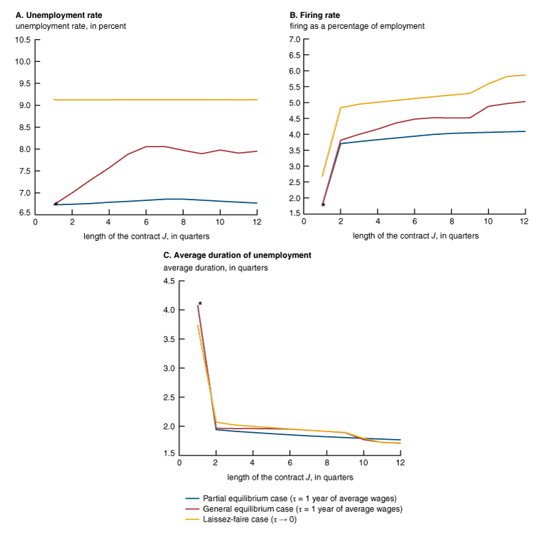
Panel A of figure 2 shows the effects on the unemployment rate ur = U/(U + N). While the fraction of agents who search U is increasing with the lengthening of the temporary contracts, we see that the unemployment rate initially increases with J but then displays a nonmonotonic behavior. We also see that the unemployment rate is almost 2.5 percentage points higher in the laissez-faire case than in the benchmark J = 1 case and that with temporary contracts of three years’ duration (J = 12) the unemployment rate is 1.2 percentage points higher than in the benchmark case. Thus, temporary contracts of three years’ duration, which are similar to those introduced by the 1984 Spanish reform, are able to close about half of the gap with the laissez-faire case.16 Figure 2, panel A also shows that the equilibrium effects on U are crucial for generating the higher unemployment rates: The effects on the unemployment rate are nonmonotonic and small in the partial equilibrium case.17
To better understand the effects on the unemployment rate (figure 2, panel A), it is helpful to decompose them into firing rate effects (figure 2, panel B) and average duration of unemployment effects (figure 2, panel C). Panel B of figure 2 shows the effects on the firing rate fr, defined as total firing divided by total employment. Recall that for the laissez-faire and partial equilibrium cases, the values of U and \(\unicode{x03B8} \) are the same across all J. As should be expected, the firing rates for the laissez-faire case are higher than the ones for the partial equilibrium case for all values of J. Notice that the firing rates in these two cases are increasing with the rise in J, including a large jump at J = 2. To understand this pattern, we concentrate on the laissez-faire case, where the employment on each island stays constant. Recall that we compute employment by tenure in the laissez-faire case as the limit for an equilibrium with \(\unicode{x03C4} \to 0\). The increase in the firing rate helps to avoid the (arbitrarily small) separation tax. The firing rate jumps between J = 1 and J = 2 because when J = 2, the temporary workers with longest tenure are fired and replaced by newly arrived workers. This reshuffling cannot be done when J = 1. The smooth increase in the firing rate with J is due to the fact that with higher J, firms can accumulate a larger proportion of their workforce as temporary workers. With this larger proportion, if they need to decrease total employment, they can do so at the same time that they hire newly arrived workers. Notice that the pattern of firing rates as a function of J for the partial equilibrium case, with substantial separation costs (one year of average wages), is generally the same as in the laissez-faire case, with essentially zero firing taxes.
As seen in figure 2, panel B, the value for the firing rate in the general equilibrium case lies in between the value for the partial equilibrium case and the one for the laissez-faire case, and it gets closer to the one for the laissez-faire case as J increases. Since in general equilibrium firms receive a higher flow of newly arrived workers (that is, a higher U), they can engage more in the replacement of temporary workers with high tenure for newly arrived workers to save on separation costs.
The quarterly firing rate for the general equilibrium case goes from 1.77 percent for J = 1 to 5.04 percent for J = 12, roughly similar to the values for Spain before and after 1984: García-Fontes and Hopenhayn (1996) estimate quarterly firing rates of 1.8 percent prior to the extension of temporary contracts’ length and 4.8 percent after it. The model slightly overestimates this effect. However, the effect in the model of going from J = 1 to J = 12 does not correspond exactly to Spain before and after 1984 because some temporary contracts were allowed in Spain before 1984.
Panel C of figure 2 shows the average duration of unemployment d, defined as (1/fr) ur/(1 − ur). The three cases display similar values. There is a large drop in the average duration between J = 1 (the benchmark case) and J = 2. This is the result of the increased hiring of newly arrived workers that we mentioned in our explanation of figure 2, panel B.18 Because d is similar for the three cases, it’s clear that the effects on unemployment are accounted for by the behavior of the firing rates discussed previously. Notice that, as opposed to the sharp change at J = 2 for the firing rate and average duration of unemployment (panels B and C of figure 2, respectively), the increase in the unemployment rate for the general equilibrium is smooth (panel A of figure 2). This is because for J = 2, the sharp decrease in the average duration of unemployment coincides with a sharp increase in the firing rate.
Figure 3 displays the fraction of permanent workers among all workers for the general equilibrium and laissez-faire cases. The fraction of permanent workers is higher for the general equilibrium case than for the laissez-faire case because in the general equilibrium case, firms retain more permanent workers to avoid the high separation costs. Nevertheless, the fraction of permanent workers is very similar in the two cases. Notice also that as J increases, the fraction of permanent workers decreases steadily. For J = 12, which corresponds to temporary contracts of three years, 33 percent of all workers are in temporary contracts (see the solid red line in figure 3, which indicates that when J = 12, 67 percent of workers are permanent employees). In Spain, the fraction of workers with temporary contracts went from about 11 percent before the 1984 reform to 16 percent in 1987, 22 percent in 1988, and 27 percent in 1989, before stabilizing to an average of about 33 percent during the 1990s (García-Fontes and Hopenhayn, 1996, and Toharia Cortés, 2002).
Figure 3. Share of permanent workers as a function of the length of temporary employment contracts
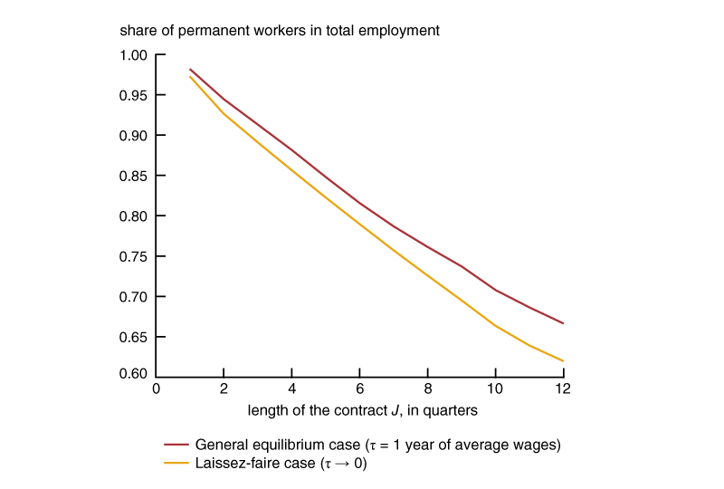
Notice that the patterns displayed in panel C of figure 2 and in figure 3 for the average duration of unemployment and the share of permanent workers among total workers are similar to the ones found in Spain after the mid-1980s. These patterns have typically been interpreted as evidence that the length of temporary contracts can play an important role in labor market dynamics. However, in our model, similar patterns are obtained for τ equal to one year of average wages, as well as for an arbitrarily small value of \(\unicode{x03C4} \)—which shows that by itself large changes in turnover do not necessarily entail large changes in welfare and other relevant variables, such as employment, unemployment, aggregate consumption, and productivity. We obtain this result under the extreme assumption that workers with different tenure are perfect substitutes. Under a different specification, such as allowing for on-the-job learning, this result will not be obtained. In particular, if the effect of on-the-job learning is large enough, a small separation cost may have a very small effect on turnover rates. Nevertheless, we interpret the spike in figure 1 for tenure of about three years as evidence that the effects of separation taxes are not completely outweighed by on-the-job learning.19 We leave the examination of a model that incorporates both features for future work.
Figure 4 shows the behavior of employment for the general equilibrium case for different values of the intertemporal substitution parameter \(\unicode{x03B3} \). As J increases, there are both income and substitution effects. The substitution effect is due to the fact that as J increases, firms have more flexibility and thus working in the market is more attractive—that is, the equilibrium value of \(\unicode{x03B8} \) increases. The income effect is due to the fact that the economy is more productive. For low values of \(\unicode{x03B3} \), the substitution effect dominates, and thus, aggregate employment increases with J. For high values of \(\unicode{x03B3} \), the income effect dominates, and thus, aggregate employment decreases with J.
Figure 4. Equilibrium employment as a function of the length of temporary employment contracts for different values of \(\unicode{x03B3} \)
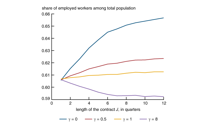
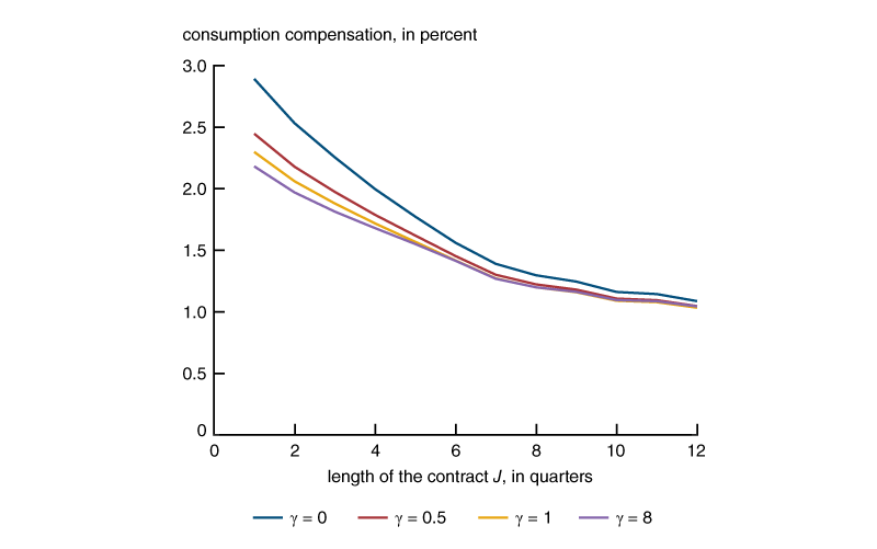
Figure 5 displays the welfare cost of temporary contracts of different lengths for different values of the intertemporal substitution parameter \(\unicode{x03B3} \). The welfare cost is measured in consumption equivalent units—that is, it is the perpetual percentage increase in consumption flow needed to make the representative household indifferent between being in the economy with temporary contracts of length J and being in the laissez-faire economy. This calculation compares the stationary equilibriums of the two economies and hence does not take into account the transition after a change in policy. Observe that for the same J, the welfare cost is always higher when the value of \(\unicode{x03B3} \) is smaller because when \(\unicode{x03B3} \) decreases, there is greater substitution between consumption and home production. However, the welfare costs are surprisingly similar across the different values of \(\unicode{x03B3} \). Interestingly, for J = 1 (the baseline case), figure 5 shows that the welfare cost of firing taxes is 2.3 percent for \(\unicode{x03B3} \text{ }=\text{ }1\) (the case of logarithmic preferences). This number is extremely similar to the one found by Hopenhayn and Rogerson (1993) and Veracierto (2001) under identical preferences. As J increases, the welfare cost decreases: The welfare cost goes from 2.3 percent for a contract length of one quarter and decreases smoothly with J until a value of around 1 percent for a contract length of three years, or J = 12. Thus, even if some characteristics of the allocation (such as the unemployment rate in figure 2, panel A) do not converge monotonically to their laissez-faire values as J increases, the welfare cost—which in a sense takes all the relevant features into consideration—does converge monotonically. The same is true for all values of the intertemporal substitution parameter \(\unicode{x03B3} \).
Figure 5. Welfare costs of temporary employment contracts of different lengths for different values of \(\unicode{x03B3} \)
Conclusion
In this article, we considered the equilibrium search model described in Alvarez and Veracierto (2012), which is a version of the Lucas–Prescott islands model with undirected search and an out-of-the-labor-force state. Calibrating the model to Spain before the major labor market reform that it introduced in 1984, we explored the quantitative effects of introducing temporary employment contracts of various lengths. An important finding of the article is that introducing temporary contracts of three years’ duration—the magnitude introduced by the 1984 Spanish reform—provides about 50 percent as much labor market flexibility as moving to a laissez-faire regime (with zero firing costs). We base this claim about the effects of temporary contracts on two key statistics—the unemployment rate, which summarizes labor reallocation, and welfare, which summarizes the overall effects on the economy of introducing such contracts.
Notes
1 Typically, termination based on economic grounds does not exempt employers from paying severance payments. Severance payments are the largest when the termination happens without cause.
2 In what follows, it may be useful to consider home as a special location (separate from the production islands) where agents can always go in order to obtain home production.
3 We refer to the tenure of a worker as the number of periods that the worker has been present on the island. For instance, a recently arrived worker has a tenure of zero periods.
4 If firing taxes applied at the firm level (instead of the island level), exactly the same competitive allocation would be obtained if employment contracts were allowed to be multiperiod and state-contingent (see Alvarez and Veracierto, 2012). Thus, the assumption that the firing taxes apply at the island level does not represent a loss in realism, but it allows for a much simpler description of a competitive equilibrium.
5 While we evaluate the role of fixed-term contracts in adding flexibility to firms’ labor adjustments, we abstract from their potential role in allowing employers to test the quality of their new workers at a reduced cost (in our model, workers are identical).
6 The type of an island is given by its current state (to be described in the second paragraph of the next section).
7 Observe that the behavior of the unemployment rate will generally differ from the behavior of \({{U}_{t}}\) because of differences in the behavior of \({{L}_{t}}\).
8 The assumptions that all search is undirected and that agents are fully insured, while extreme, will play an important role in keeping the model tractable.
9 Actually, the saving from avoiding firing taxes does not equal the full amount \(\unicode{x03C4} \) saved during the current period because the worker may be fired the following period.
10 When J = 1, the dismissal of anyone who has worked, even for one period, triggers the separation tax \(\unicode{x03C4} \text{ }>\text{ }0\). Thus, there are no temporary workers in this case.
11 Observe that, independent of \(\unicode{x03C4} \) being large or small, a contracting island will always remove the workers with tenure J − 1 first, then those with tenure J − 2, and so on until it removes those with tenure 1. Only after all workers with tenure 1 have been removed will the island start removing permanent workers (those with tenure J). Thus, the hiring and firing rates across the different tenure levels are well determined.
12 These reforms were partially undone during the 1990s, when the maximum length of fixed-term contracts was reduced from three years to one year and the severance payments for ordinary indefinite-length contracts were substantially reduced. However, even after this partial reversal, the fraction of workers under fixed-term contracts stabilized at about 33 percent (see Toharia Cortés, 2002, figure 1, p. 119).
13 In Alvarez and Veracierto (2000), we analyzed the effects of introducing unemployment insurance (UI) benefits into the model with firing taxes. Introducing UI benefits of the magnitude observed in Spain increases the unemployment rate by roughly 10 percent and more than doubles the average duration of unemployment (see subsection 4.4.1 on UI benefits, firing subsidies, firing taxes, and severance payments, as well as table 5, of Alvarez and Veracierto, 2000, pp. 284–285, 298).
14 The different combinations of \(\left( \unicode{x03B3} ,\text{ }\unicode{x03C9} \right)\) are: (0, 1.3047), (1/2, 1.0739), (1, 0.883), and (8, 0.058). With \(\unicode{x03B3} \text{ }=\text{ }0\), there are no income effects, since preferences are linear. With \(\unicode{x03B3} \text{ }=\text{ }1\), income and substitution effects of a permanent increase in wages cancel each other out. With \(\unicode{x03B3} \text{ }=\text{ }8\), the income effect is much higher, so that the uncompensated labor supply elasticity is lower, similar to the values estimated by Nickell (1997).
15 Because of the decreasing returns to scale at the island level, the higher value for U reduces the value of an additional worker at every island and restores the general equilibrium at \(\unicode{x03B8} \text{ }=\text{ }\unicode{x03C9} /\left( 1\text{ }-\text{ }\unicode{x03B2} \right)\).
16 In the data the relationship between unemployment and temporary contracts is not as clear. However, Dolado, García-Serrano, and Jimeno (2002, p. F285) survey the literature and conclude that the introduction of temporary contracts in Spain had a “neutral or slightly positive effect on unemployment.”
17 These partial equilibrium effects are consistent with previous findings in the literature: We know at least since Bentolila and Bertola (1990) that the effects of firing costs on average employment are ambiguous in that setting.
18 To better understand what is happening in our model, it may be useful to consider the case of an island that would like to have the same total employment level that it had during the previous period. When J = 1, the island will not hire any of the new arrivals U (since replacing permanent workers with new arrivals would involve paying firing taxes). However, when J = 2 the island will want to replace all the workers with tenure j = 1 with new arrivals in order to avoid the j = 1 workers from becoming permanent workers. For this reason, it is harder to transit out of unemployment under J = 1 than under J = 2. This is also the reason why the firing rate jumps up from when J = 1 to when J = 2 in figure 2, panel B. Even when the firing taxes are arbitrarily small, the temporary contracts induce the islands to churn their workers quite significantly.
19 With on-the-job learning and firing costs, if the effect of learning is strong enough, it will not be optimal for the firm to fire first the temporary workers with higher tenure. In this case, the spike at the end of the fixed-term contracts shown for Spain in figure 1 would not be obtained.
Appendix: Calibration of \(\unicode{x03C4} \)
Heckman and Pagés (2000) propose to summarize employment protection policies into a single statistic. The measure they use is the expected discounted cost, at the time that a worker is hired, of dismissing the worker in the future. Their index I is given by
\[I=\sum\limits_{t=1}^{T}{{{\unicode{x03B2} }^{t}}{{\unicode{x1E9F} }^{t-1}}\left( 1-\unicode{x1E9F} \right)}\left\{ {{b}_{t}}+aS_{t}^{j}+\left( 1-a \right)S_{t}^{u} \right\},\]
where T is the maximum tenure considered in the index, \(\unicode{x03B2} \) is a time discount factor, \(\unicode{x1E9F} \) is the survival rate (probability of remaining employed next period if employed during the current period), \({{b}_{t}}\) is the wage earned during the advance-notice period for a worker of tenure \(t, a\) is the probability that a dismissal is considered “justified” (that is, “fair” or “objective”), \(S_{t}^{j}\) is the severance payment to a worker of tenure t if the dismissal is classified as “justified,” and \(S_{t}^{u}\) is the severance payment to a worker of tenure t if the dismissal is “not justified.”
Heckman and Pagés (2000) use a year as the time period, along with the following values: \(\unicode{x03B2} =\text{ }0.92\) (an 8 percent interest rate), \(\unicode{x1E9F} =\text{ }0.88\) (a turnover rate of 12 percent, based on data for the United States), and a value of T of 20 years; in addition, for Spain they advocate for using \(a\) = 0.2 for the period before 1997, based instead on the information from Bertola, Boeri, and Cazes (2000). Heckman and Pagés (2000) compute their job security index for Spain in the late 1990s. Since we calibrate our model to the period before the broadening in the applicability of temporary contracts, we recompute their index for the policies in place before the 1984 labor market reform. We use the following values:
- \({{b}_{t}}\): one month of wages for tenure 1 and two and three months for higher tenure (Organisation for Economic Co-operation and Development, 1999, table 2.2, p. 57);
- \(a\): 0.2 (since their argument applies prior to 1984);
- \(S_{t}^{j}:\) two-thirds months per year, up to a maximum of 12 months (Organisation for Economic Co-operation and Development, 1999, table 2.A.2, p. 96); and
- \(S_{t}^{u}:\) one and a half months per year, up to a maximum of 42 months (Organisation for Economic Co-operation and Development, 1999, table 2.A.5, p. 101).
We consider two cases. The first case is as follows: With these choices for \({{b}_{t}}\), \(a\), \(S_{t}^{j}\), and \(S_{t}^{u}\), along with the values for \(\unicode{x03B2} \) and \(\unicode{x1E9F} \) used by Heckman and Pagés (2000), we obtain a value of I prior to 1984 of 0.42 as a fraction of annual average wages. And the second case is the following: If instead we use \(\unicode{x03B2} =\text{ }0.96\), which is the same value we use in our main text discussion, and \(\unicode{x1E9F} =\text{ }0.93\), which is closer to the one for Spain prior to 1984 according to Cabrales and Hopenhayn (1997), we obtain a value of I prior to 1984 of 0.56 as a fraction of annual average wages.
Finally, since in our benchmark case the firing taxes do not depend on the tenure of the workers, we select the value of \(\unicode{x03C4} \) so that the value of the index I will yield the value we calibrate for Spain prior to the 1984 reform. This value solves the equation:
\[I=\sum\limits_{t=1}^{T}{{{\unicode{x03B2} }^{t}}{{\unicode{x1E9F} }^{t-1}}\left( 1-\unicode{x1E9F} \right)}\,\unicode{x03C4} =\unicode{x03C4} \left( 1-\unicode{x1E9F} \right)\,\,\unicode{x03B2} \frac{1-{{\left( \unicode{x03B2}\unicode{x1E9F}\right)}^{T}}}{1-\unicode{x03B2} \unicode{x1E9F} }\]
or
\[\unicode{x03C4} =I\,\frac{1-\unicode{x03B2} \unicode{x1E9F} }{\left( 1-\unicode{x1E9F} \right)\,\unicode{x03B2} \,\left( 1-{{\left( \unicode{x03B2} \unicode{x1E9F} \right)}^{T}} \right)}.\]
The value of \(\unicode{x03C4} \) that corresponds to the first case is 0.74 of annual average wages, and the value of \(\unicode{x03C4} \) that corresponds to the second case is 0.98 of annual average wages. We think that for our purposes the choices of the second case better reflect the situation prior to 1984 in Spain, and hence, we calibrate the model to \(\unicode{x03C4} \) equivalent to one year of average wages.
References
Aguirregabiria, Victor, and Cesar Alonso-Borrego, 2014, “Labor contracts and flexibility: Evidence from a labor market reform in Spain,” Economic Inquiry, Vol. 52, No. 2, April, pp. 930–957. Crossref
Alvarez, Fernando, and Marcelo Veracierto, 2012, “Fixed-term employment contracts in an equilibrium search model,” Journal of Economic Theory, Vol. 147, No. 5, September, pp. 1725–1753. Crossref
Alvarez, Fernando, and Marcelo Veracierto, 2000, “Labor-market policies in an equilibrium search model,” in NBER Macroeconomics Annual 1999, Ben S. Bernanke and Julio J. Rotemberg (eds.), Vol. 14, Cambridge, MA: MIT Press, pp. 265–304. Crossref
Bentolila, Samuel, and Giuseppe Bertola, 1990, “Firing costs and labour demand: How bad is Eurosclerosis?,” Review of Economic Studies, Vol. 57, No. 3, July, pp. 381–402. Crossref
Bentolila, Samuel, and Gilles Saint-Paul, 1992, “The macroeconomic impact of flexible labor contracts, with an application to Spain,” European Economic Review, Vol. 36, No. 5, June, pp. 1013–1047. Crossref
Bertola, Giuseppe, Tito Boeri, and Sandrine Cazes, 2000, “Employment protection in industrialized countries: The case for new indicators,” International Labour Review, Vol. 139, No. 1, March, pp. 57–72. Crossref
Blanchard, Olivier, and Augustin Landier, 2002, “The perverse effects of partial labour market reform: Fixed-term contracts in France,” Economic Journal, Vol. 112, No. 480, June, pp. F214–F244. Crossref
Buddelmeyer, Hielke, Gilles Mourre, and Melanie E. Ward-Warmedinger, 2004, “Recent developments in part-time work in EU-15 countries: Trends and policy,” IZA (Institute of Labor Economics), discussion paper, No. 1415, November, available online.
Cabrales, Antonio, and Hugo A. Hopenhayn, 1997, “Labor-market flexibility and aggregate employment volatility,” Carnegie-Rochester Conference Series on Public Policy, Vol. 46, June, pp. 189–228. CrossrefCahuc, Pierre, and Fabien Postel-Vinay, 2002, “Temporary jobs, employment protection and labor market performance,” Labour Economics, Vol. 9, No. 1, February, pp. 63–91. Crossref
Dolado, Juan J., Carlos García-Serrano, and Juan F. Jimeno, 2002, “Drawing lessons from the boom of temporary jobs in Spain,” Economic Journal, Vol. 112, No. 480, June, pp. F270–F295. Crossref
García-Fontes, Walter, and Hugo Hopenhayn, 1996, “Flexibilización y volatilidad del empleo,” Moneda y Crédito, No. 202, pp. 205–227, available online.
Güell, Maia, and José Vicente Rodríguez Mora, 2010, “Temporary contracts, incentives and unemployment,” Centre for Economic Policy Research, discussion paper, No. DP8116, November, available online.
Heckman, James J., and Carmen Pagés, 2000, “The cost of job security regulation: Evidence from Latin American labor markets,” National Bureau of Economic Research, working paper, No. 7773, June. Crossref
Hopenhayn, Hugo, and Richard Rogerson, 1993, “Job turnover and policy evaluation: A general equilibrium analysis,” Journal of Political Economy, Vol. 101, No. 5, October, pp. 915–938. Crossref
Lucas, Robert E., Jr., and Edward C. Prescott, 1974, “Equilibrium search and unemployment,” Journal of Economic Theory, Vol. 7, No. 2, February, pp. 188–209. Crossref
Nickell, Stephen, 1997, “Unemployment and labor market rigidities: Europe versus North America,” Journal of Economic Perspectives, Vol. 11, No. 3, Summer, pp. 55–74. Crossref
Organisation for Economic Co-operation and Development, 1999, OECD Employment Outlook: June 1999, report, Paris, June, available online.
Toharia Cortés, Luis, 2002, “El modelo español de contratación temporal,” Temas Laborales, No. 64, pp. 117–139, available online.
Veracierto, Marcelo, 2007, “On the short-run effects of labor market reforms,” Journal of Monetary Economics, Vol. 54, No. 4, May, pp. 1213–1229. Crossref
Veracierto, Marcelo, 2001, “Employment flows, capital mobility, and policy analysis,” International Economic Review, Vol. 42, No. 3, August, pp. 571–596. Crossref


