

Introduction and summary
In the first quarter of 2020, as the scale of the Covid-19 crisis became apparent, equity indexes in the United States endured one of their most dramatic deteriorations in history. By August of that year, however, the stock market had bounced back, and the rally continued apace all the way into late 2021. While a number of developments likely contributed to the rebound—including Federal Reserve liquidity support, fiscal stimulus, and the development of vaccines—one factor that has received particular attention is the extraordinarily accommodative monetary policy that the Fed adopted during this period. At the onset of the crisis, the Federal Open Market Committee (FOMC) slashed the federal funds rate’s target range to near zero, and it subsequently purchased over $4 trillion of U.S. Treasury and mortgage-backed securities.1 These actions lowered interest rates and supported the economic recovery while also likely having an outsized effect on asset prices, including the prices of equities. Similarly, when policymakers began to signal the removal of accommodation around the end of 2021, equity prices sputtered.
In this article I present a case study of the relationship between monetary policy, long-term interest rates, and the stock market by unpacking these developments. In general, monetary policy has three distinct effects on stock prices. First, by stimulating the macroeconomy, accommodative policy raises corporate profits, increasing the expected cash flows of equity claims. Second, by lowering the term structure of interest rates, or yield curve, accommodation reduces the risk-free rate at which dividends are discounted, boosting their present value. Finally, loosening monetary policy may lower risk premiums by helping to remove tail risk (that is, the chance of severe adverse movements in asset prices or an economic crisis) and by relieving financial institutions’ balance-sheet constraints, through the “risk-taking channel.”2 I explore how important each of these three mechanisms was in supporting the growth of equities during the period of policy easing following the onset of the pandemic.
My analysis proceeds in two steps. First, using an extension of the Campbell–Shiller dividend-discount model (Campbell and Shiller, 1988a, 1988b), where expected profits are estimated by a vector autoregression (VAR), I decompose total stock market changes in each quarter after the peak of the market in early 2020 into changes resulting from expected earnings and discount rates (that is, the future expected rates of return that investors require on equities given their risk profiles). Consistent with evidence from this type of model from before the Covid period, I find that most stock market fluctuations were not primarily driven by profit expectations but rather by discounting. My model allows me to go beyond the Campbell–Shiller model by further separating discount factors into a risk-free component and a residual component that embeds the equity risk premium (ERP). I find that while shifts in risk-free discount rates and expected profits had large effects on the stock market at times, most of the early drop in stock prices and a significant fraction of the subsequent recovery were due to fluctuations in the component containing risk premiums.
This decomposition does not tell us how much of the stock market dynamics over this period resulted from monetary policy, given that monetary policy can affect all three components of stock prices. To answer that question, the second stage of the analysis identifies monetary policy shocks within the VAR. The identification uses sign restrictions on the three components of stock prices to sweep out effects that might result from the Fed conveying information about underlying macroeconomic fundamentals or its reaction function to economic news, rather than from changes in policy per se. I use the results to construct a counterfactual scenario in which the Fed maintained medium-term U.S. Treasury yields at their pre-Covid level throughout the Covid period. I focus on medium-term yields because short-term rates were constrained by the effective lower bound throughout this period and the Fed operated further out the yield curve by using forward guidance and large-scale asset purchases.3 The exercise shows that if policy had maintained five-year Treasury yields at their pre-Covid level, stock prices nine months after the onset of the pandemic would have been 37% lower than observed, with the effects operating through all three components. These effects gradually reversed as markets priced in the anticipation of policy tightening. By the time policy liftoff occurred in March 2022, longer-term Treasury yields had exceeded their pre-Covid levels, and the model implies that monetary policy had become a net drag on the stock market, again operating roughly equally through all three components.
These results are of interest for several reasons. First, they show that monetary policy can be an effective tool in stabilizing financial markets during crises. Although I do not directly examine the macroeconomic effects of Covid-era monetary policy, the stock market is an important channel through which households accumulate purchasing power and businesses finance themselves, and I show that monetary policy supported it significantly. Second, the results highlight that monetary policy does not necessarily exert all of its effects through corporate profits or risk-free rates as one might expect. Policy shocks do not have large effects on expected real profits many years in the future or on long-term yields, but these distant-horizon objects loom large in equity valuations. Rather, the results are qualitatively consistent with previous studies that suggest significant changes in the equity risk premium in response to FOMC actions—such as Bernanke and Kuttner (2005), Bekaert, Hoerova, and Lo Duca (2013), Cieslak and Pang (2021), and Bauer, Bernanke, and Milstein (2023)— and are consistent with an important role for the risk-taking channel.
Several other papers have presented decompositions of stock market movements during the Covid crisis using various methodologies, with a particular focus on the large gyration in the first half of 2020. Gormsen and Koijen (2020) and Knox and Vissing-Jorgensen (2022) use information from dividend strips, while Landier and Thesmar (2020) rely on analysts’ earnings forecasts. Cox, Greenwald, and Ludvigson (2020) use a method similar to what I have adopted for this article, but their approach features more structure on the discount rate. Broadly consistent with my findings here, all of these papers conclude that the large movements in early 2020 were primarily due to discount rates. However, none of them explicitly examines the role of monetary policy in driving these changes. All of them also stop short of analyzing the significant further developments in the stock market and monetary policy through early 2022. Separately, there is a long tradition examining the extent to which monetary policy affects the stock market, dating back to at least to Gürkaynak, Sack, and Swanson (2005) and Rigobon and Sack (2004). This article is in that tradition, but it extends the methodology by examining the effects on the three components of stock prices noted previously. It also incorporates recent insights into the potential for Fed information effects (Nakamura and Steinsson, 2018; and D’Amico and King, 2023b) that may bias other estimates.
Unconditional decomposition of equity prices
In this section, I explain how I decompose total stock market changes in each quarter between early 2020 and early 2022. First, I discuss my conceptual framework for studying changes in equity prices by decomposing them into changes in the three components. Then I explain the estimation of my VAR model, which provides an important input into this decomposition.
Conceptual framework
I begin by decomposing changes in equity prices into changes in three components: 1) risk-free discount rates, 2) expected future earnings, and 3) a residual term reflecting risk premiums and other factors. By definition, the risk-free discount rate for a cash flow n periods ahead is given by $ \unicode{x03B4} _{t}^{(n)}=\,\exp\left[ -ny_{t}^{(n)} \right],$ where $y_{t}^{(n)}$ is the zero-coupon riskless bond yield. Thus, for an equity contract with a claim to an infinite future stream of profits $\{{{\unicode{x03A0} }_{t}}\},$ I can define the risk-free present value of the expected cash flow stream as follows:
$1)\quad{{V}_{t}}=\sum\limits_{n=0}^{\infty }{ \unicode{x03B4} _{t}^{(n)}{{\mathrm{E}}_{t}}}\left[ {{\prod }_{t+n}} \right],$
where Et denotes the expected value conditional on information at time t. Letting st denote the log of the market price of the equity claim, one can write
$2){\quad}s_t\ = {\mathrm{log}\ V}_t\ -\ {ERP}_t,$
where ERPt is the equity risk premium. This equation defines the equity risk premium for the purposes of this article. It is the difference between the riskless discounted value of future cash flows and their current price.4
Substituting equation 1 into equation 2 and taking a first-order Taylor series expansion gives the approximate log change in the stock price over a period:
$3)\quad\unicode{x0394} {{s}_{t}}\approx \frac{1}{{{V}_{t-1}}}\sum\limits_{n=0}^{\infty }{\unicode{x0394} \unicode{x03B4} _{t}^{(n)}{{\mathrm{E}}_{t-1}}\left[ {{\prod }_{t+n}} \right]}+\frac{1}{{{V}_{t-1}}}\sum\limits_{n=0}^{\infty }{ \unicode{x03B4} _{t-1}^{(n)}}\left( {{\mathrm{E}}_{t}}\left[ {{\prod }_{t+n}} \right]-{{\mathrm{E}}_{t-1}}\left[ {{\prod }_{t+n-1}} \right] \right)-\unicode{x0394} ER{{P}_{t}}.$
This shows that stock returns can in principle be decomposed into three parts. The first term is a change in risk-free discounting of a given expected profit stream; the second term is a change in expectations of the profit stream itself, holding the discount rate constant; and the third term is a change in the risk premium. To understand a change in stock prices over a given period, one can try to measure each of these components. The approach is reminiscent of Campbell and Shiller (1988a, 1988b), although in those papers the authors do not separate risk-free rates from risk premiums. This is a key distinction for this article because the effects of monetary policy on Treasury yields may be quite different from its effects on the compensation investors demand for risk.
Note that, if investors expected the economy to grow faster than their risk-free discount rate in the long run, they would bid up Vt to an infinite value. For the calculation of the level of Vt to make sense, it must therefore be the case that at a long enough horizon, discount rates are always higher than expected profit growth, a restriction I impose in the estimation. The result that far-forward bond yields are greater than long-run rates of economic growth holds in a fairly broad set of asset-pricing models under standard parameterizations, as discussed in the accompanying box. However, even if the condition does not hold in reality, the decomposition in equation 3 can still be viewed as an approximation that holds when calculated over finite horizons.
Box 1. Long-term yields and growth in a simple model
For the model presented in this article, it is assumed that long-term bond yields are always greater than long-run rates of profit growth. While there is no guarantee that this condition must hold in the economy, I demonstrate here the conditions under which it is the case in a commonly used consumption-based asset-pricing model.
Suppose consumers have preferences over real consumption Ct with constant relative risk aversion. Let β be the rate of time preference, γ be the risk-aversion coefficient, and Pt be the price level. The nominal discount function (or bond price) for such an economy, reflecting the present value of a dollar delivered with certainty n periods from now, is given by
\[\begin{align} \unicode{x03B4} _{t}^{(n)}& ={{\unicode{x03B2} }^{n}}{{\text{E}}_{t}}\left[ {{\left( \frac{{{C}_{t+n}}}{{{C}_{t}}} \right)}^{-\unicode{x03B3} }}\frac{{{P}_{t}}}{{{P}_{t+n}}} \right] \\ & ={{\unicode{x03B2} }^{n}}{{\text{E}}_{t}}\left[ \exp \sum\limits_{m=1}^{n}{\left( -\unicode{x03B3} {{g}_{t+m}}-{{\unicode{x03C0} }_{t+m}} \right)} \right], \\ \end{align}\]
where Et denotes the expected value conditional on information at time t, gt is the rate of real consumption growth, and πt is the rate of inflation.
The infinite-horizon nominal bond yield in this model is, by definition, \[y_{t}^{(\infty )}=\,\,\,\underset{n\to \infty }{\mathop{\lim }}\,-\frac{1}{n}\log \unicode{x03B4} _{t}^{(n)}.\] Supposing permanent innovations in consumption and prices to be log-normal, this becomes \[y_{t}^{(\infty )}={{\unicode{x03C0} }^{*}}+\unicode{x03B3} {{g}^{*}}-\log \unicode{x03B2} -\frac{1}{2}\left( {{\unicode{x03B3} }^{2}}\unicode{x03C3} _{c}^{2}+\unicode{x03C3} _{p}^{2} \right),\] where g∗ and π* are the long-run rates of growth and inflation, respectively; $\unicode{x03C3} _{c}^{2}$ is the conditional variance of the stochastic trend in log Ct ; $\unicode{x03C3} _{p}^{2}$ is the conditional variance of the stochastic trend in log Pt; and I have assumed for the sake of simplicity that any trends in consumption and prices are uncorrelated.
From this expression, it is clear that infinite-horizon nominal bond yields are greater than long-run nominal growth $\left( y_{t}^{(\infty )}>{{\unicode{x03C0} }^{*}}+{{g}^{*}} \right)$ whenever
$\text{B}1)\quad\left( \unicode{x03B3} -1 \right){{g}^{*}}-\log \unicode{x03B2} >\frac{1}{2}\left( {{\unicode{x03B3} }^{2}}\unicode{x03C3} _{c}^{2}+\unicode{x03C3} _{p}^{2} \right).$
This inequality holds under a wide range of plausible parameter values. Moreover, the requirement that equity prices be finite implies further restrictions on the values of parameters that are admissible. In particular, consider contracts (“Lucas trees”) paying dividends Dt equal to nominal consumption. Their price is
\[\begin{align} {{S}_{t}}& =\sum\limits_{n=0}^{\infty }{{{\unicode{x03B2} }^{n}}{{\text{E}}_{t}}\left[ {{\left( \frac{{{C}_{t+n}}}{{{C}_{t}}} \right)}^{-\unicode{x03B3} }}{{D}_{t+n}} \right]} \\ & ={{D}_{t}}\sum\limits_{n=0}^{\infty }{{{\unicode{x03B2} }^{n}}{{\text{E}}_{t}}}\left[ \exp \left( 1-\unicode{x03B3} \right)\left( {{g}_{t+1}}+\ldots +{{g}_{t+n}} \right) \right]. \\ \end{align}\]
This infinite sum converges if and only if $(\unicode{x03B3} -1){{g}^{*}}-\log\unicode{x03B2} >0.$ One implication is that if the economy is trend stationary, so that $\unicode{x03C3} _{c}^{2}=\unicode{x03C3} _{p}^{2}=0,$ the B1 inequality is always satisfied. More generally, the condition is only violated in cases involving very volatile stochastic trends. For example, under typical annual parameter values of $\unicode{x03B2} =0.96$, $\unicode{x03B3} =2$, and ${{g}^{*}}=0.02$ and conservatively high values of ${{\unicode{x03C3} }_{c}}={{\unicode{x03C3} }_{p}}=\text{ }1$%, the left-hand side of the B1 inequality is equal to 6.08%, while the right-hand side is equal to just 0.03%.a
a Models with recursive preferences place higher weight on long-run outcomes, boosting the effects of the variance terms in the B1 inequality, and thus are more likely to lead to the nonexistence of Vt in the presence of stochastic trends.
Estimation
Because equity prices are claims to nominal cash flows, all variables in the model are in nominal terms and discounted at nominal rates.5 Risk-free discount rates $ \unicode{x03B4} _{t}^{(n)}$ can be computed directly from the nominal Treasury yield curve. To measure expected nominal profits, I use forecasts from a VAR model. The same VAR will be used to identify and trace out the dynamic effects of monetary policy shocks, discussed in the next section. The “risk premium” ERPt is treated as a residual—it is the movement in stock prices that cannot be accounted for by changes in risk-free rates or expected profits. The method of using a VAR to estimate expected cash flows follows Campbell and Shiller (1988a, 1988b) and other subsequent work. One caveat to such an approach is that if market participants have in mind a different model for forecasting profits than the VAR, changes in ERPt may reflect this misspecification in addition to embedding the true equity risk premium.6
The VAR contains the one-year, five-year, and 30-year zero-coupon Treasury yields from the Gürkaynak, Sack, and Wright (2007) data set, the log first difference of after-tax corporate profits from the U.S. Bureau of Economic Analysis’s (BEA) National Income and Product Accounts of the United States (NIPAs), and the log first difference of the FT Wilshire 5000 total return equity index. The model is estimated using data at a quarterly frequency, from the first quarter of 1990 through the second quarter of 2022. To reduce short-term noise in the asset price series, I measure quarter-end stock and bond prices using the averages of the daily values over the final month of each quarter.
In order to discipline the model, I impose two restrictions on the reduced-form specification. First, I assume that stock prices and corporate profits are co-integrated, a standard assumption in the asset-pricing literature. Operationally, this involves including the difference between the log levels of the two series as a variable in the VAR (making it a vector error-correction model). Second, I impose that the long-run growth of profits cannot be greater than the steady-state value of the long-term interest rate. As noted, this condition is necessary for the risk-free discounted component of stock prices to exist. In order to operationalize it, I estimate the VAR by Bayesian methods, sample repeatedly from the posterior distribution of parameters, and use rejection sampling to exclude parameter draws that violate the inequality. Details about how the VAR is estimated are contained in the appendix.
1. Decomposition of stock returns during the Covid period
| Decomposition of stock returns | ||||
|---|---|---|---|---|
| Time period | Log change in stock price | Expected nominal profits | Risk-free discounting | Residual/risk premium |
| Initial shock and policy response
December 2019–March 2020 |
–0.19 | –0.08 [–0.16, 0.02] |
+0.18 [0.17, 0.19] |
–0.30 [–0.39, –0.21] |
| Rebound March–September 2020 |
+0.25 | +0.19 [0.13, 0.24] |
+0.03 [0.03, 0.03] |
+0.03 [–0.03, 0.09] |
| Continuing recovery September 2020–December 2021 |
+0.34 | +0.25 [0.19, 0.31] |
–0.12 [–0.12, –0.11] |
+0.20 [0.14, 0.26] |
| Beginning of policy tightening December 2021–March 2022 |
–0.07 | –0.01 [–0.06, 0.04] |
–0.16 [–0.16, –0.14] |
+0.10 [0.04, 0.15] |
Using the observed yield curve and VAR-based profits forecasts at each point in time, I compute the first two sums in equation 3 through 800 quarters in the future.7 Based on these calculations, figure 1 shows the decomposition of log changes in the stock market since December 2019, just before the pandemic began to weigh on U.S. markets. I focus on four subsequent points in time: 1) March 2020, in the immediate aftermath of the shock; 2) September 2020, at which point I estimate monetary policy to have had its largest effect on stock prices; 3) December 2021, by which point the economy had largely recovered to pre-pandemic levels, but policymakers had not yet begun to actively tighten policy; and 4) March 2022, after the FOMC had stopped expanding its balance sheet and begun to raise short-term rates. For reference, the blue lines in figures 2 and 3 show the observed paths of Treasury yields and stock prices.
2. Observed and counterfactual paths of U.S. Treasury bond yields
A. One-year yield
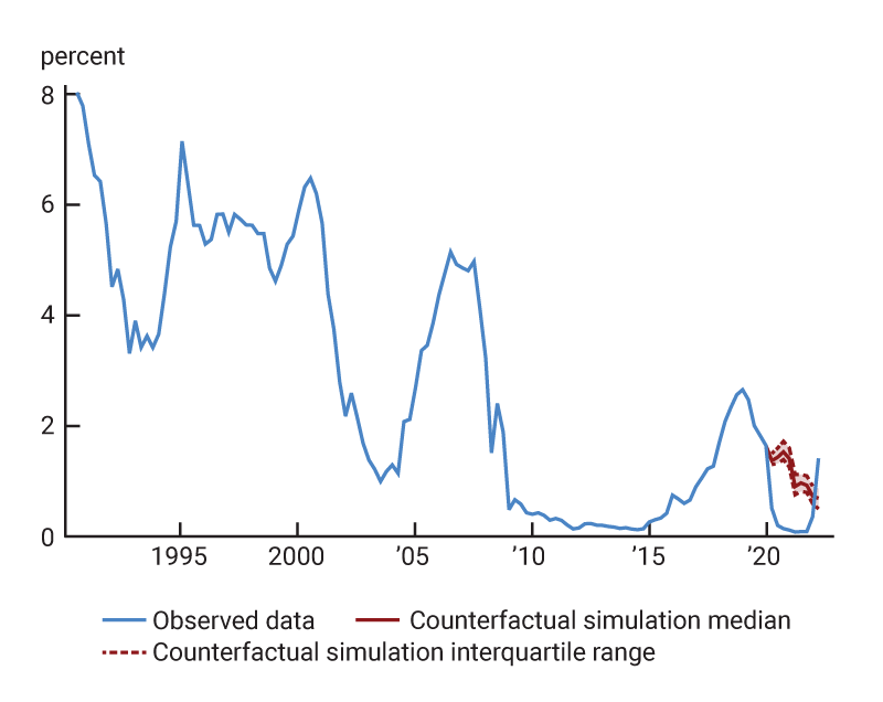
B. Five-year yield
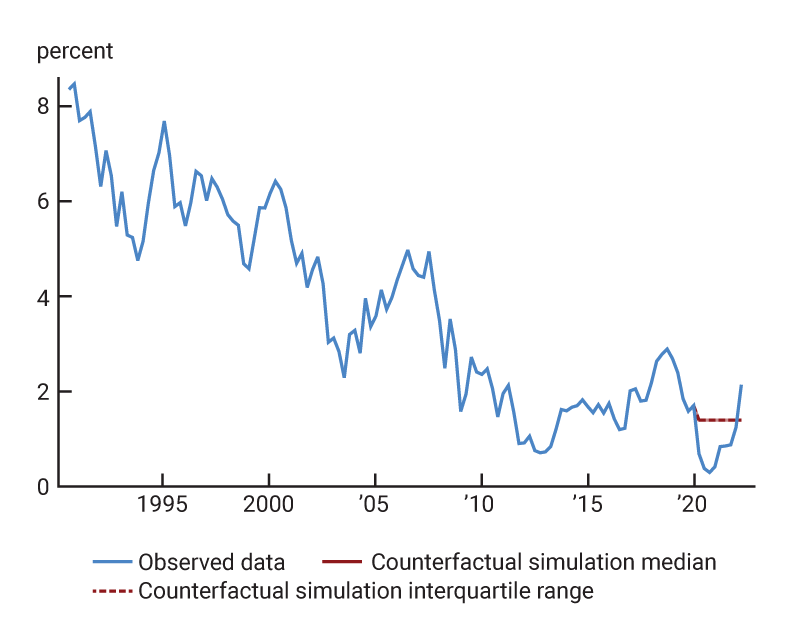
C. 30-year yield
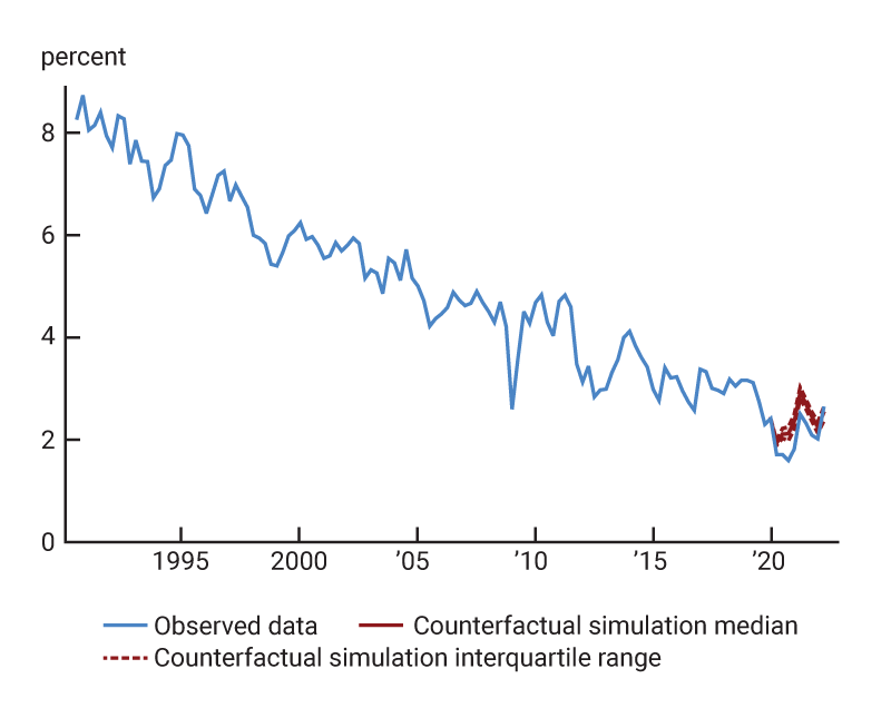
Sources: Author’s calculations based on data from the U.S. Bureau of Economic Analysis, National Income and Product Accounts of the United States, from the Federal Reserve Bank of St. Louis, FRED; and Gürkaynak, Sack, and Wright (2007).
3. Observed and counterfactual paths of stock prices
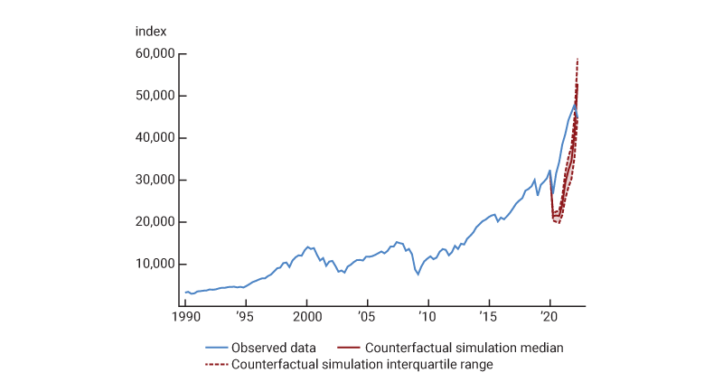
Sources: Author’s calculations based on data from the U.S. Bureau of Economic Analysis, National Income and Product Accounts of the United States, and FT Wilshire 5000 Index from the Federal Reserve Bank of St. Louis, FRED; and Gürkaynak, Sack, and Wright (2007).
Over the first quarter of 2020, the FT Wilshire 5000 Index declined 17% on net, corresponding to a change in log prices of –0.19. (This net decline is somewhat less dramatic than the 30% drop that occurred between mid-February and late March, which the model does not see, given the frequency of the data.) Meanwhile, as can be seen in panels A and B of figure 2, the yield curve fell significantly in response to accommodative monetary policy and expectations for lower nominal growth, with the five-year Treasury yield, for example, dropping by 101 basis points. The effect of the decline in the yield curve, all else being equal, was to boost stock prices—the calculation shows that lower yields raised log stock prices by 0.18 log points; however, this improvement was more than offset by an increase in the ERP that dragged log stock prices down by 0.30 log points (see the first row of figure 1). Thus, on balance, discount factors had a negative impact on the stock market during this three-month period. Negative expected profit growth also contributed to downward pressure on stock prices in this quarter, though less so.
Between March and September 2020, risk-free yields and risk premiums stayed nearly constant, contributing only modestly to the recovery in stock prices; however, expected profits rose, boosting stock prices by 0.19 log points relative from their early-pandemic lows (see second row of figure 1). Over the next 15 months, as the economy continued to recover from the brief but severe recession, the stock market rose an additional 41% (0.34 log points); the model shows that this growth can be attributed to roughly equal improvements in expected profits and risk premiums, with the concomitant rise in Treasury yields offsetting some of this effect through discounting (see third row of figure 1). By this point, inflation had accelerated notably, so that much of the growth in expected profits likely reflected higher consumer prices, rather than higher real earnings.
Finally, the last row of figure 1 shows where the stock market ended in March 2022. Between December 2021 and March 2022, yields continued rising in the wake of persistent inflation and the removal of policy accommodation. Indeed, except at very short maturities, the March 2022 yield curve exceeded its pre-pandemic level. Consequently, risk-free discounting subtracted a further 15% (0.16 log points) from stock prices during these three months. The expected path of nominal profits was nearly unchanged, with inflationary effects likely balancing a decline in expected real growth. These two factors more than accounted for the 0.07 decline in log stock prices actually observed during this quarter, so that, perhaps surprisingly, the model does see a modest decrease in risk premiums providing support to equity prices (equivalent to 0.10 log points) during this time.
Identifying the effects of monetary policy
I next ask how much of the changes in equity prices documented in the previous section can be explained by monetary policy during the Covid period and through which channels. As noted earlier, monetary policy affects all three components of equity returns: corporate profits, risk-free discount rates, and risk premiums. To examine how each of these components changed, I use a strategy that considers a counterfactual world in which policy held medium-term interest rates constant throughout the Covid period.
In order to simulate the effects of a counterfactual monetary policy path, one needs to identify monetary policy shocks in the VAR. There is, of course, a large literature on this topic. One important issue that has gained attention recently is that there may be different types of monetary policy shocks with different effects. For example, Nakamura and Steinsson (2018) and others have argued that monetary policy communications convey different signals and, in particular, they may reveal the Federal Reserve’s private information about the economic outlook to the market. To sweep out these effects, D’Amico and King (2023b) impose on expected interest rates, expected gross domestic product (GDP) growth, and expected inflation sign restrictions that can only be consistent with exogenous policy shocks, not with information effects. I follow a similar approach. As suggested in the introduction and summary, exogenous policy-easing shocks should 1) raise expected nominal profits, 2) cause risk-free discounting to decline, and 3) not cause risk premiums to increase. I impose these conditions to identify exogenous monetary policy shocks in the VAR. In contrast, an endogenous policy easing—in response to recessionary or deflationary developments—would typically be associated with a decrease in nominal profits or an increase in risk premiums or both.
A number of recent papers take a related approach by combining interest rate movements with sign restrictions on the stock market (for instance, Matheson and Stavrev, 2014; D’Amico, King, and Wei, 2016; and Jarocińksi and Karadi, 2020). Those papers impose restrictions on stock prices, but not on expected economic performance. Yet, it is not clear that that approach is sufficient to remove possible information effects. The Fed revealing its private information (or being perceived to do so) has an ambiguous effect on stock prices because risk-free discounting and profits move in opposite directions in response to such shocks, while the effects on risk premiums are unclear. It is thus likely that sign restrictions on stock prices and interest rates alone are not adequate to isolate exogenous policy innovations. In contrast, my restrictions ensure that information effects are excluded because they also involve expectations of future cash flows.8
Specifically, after estimating the VAR described in the previous section, I extract the vector of residuals and calculate its covariance matrix S over the sample. Since S is positive-definite and symmetric, there are an infinite number of matrices M that satisfy M′M = S. These matrices can be thought of as candidates for the contemporaneous multipliers on structural shocks that have zero means and unit variance. Without loss of generality, I designate the first row of the M as corresponding to an exogenous monetary policy shock. I then repeatedly draw random candidate matrices and check whether the elements of the first row satisfy the conditions just mentioned. In particular, I keep drawing until I have 1,000 draws for which the three components of stock returns shown in equation 3 all have the same sign.9 Finally, I follow Fry and Pagan (2011), Cieslak and Pang (2021), and others by selecting the “median target” draw (that is, the draw closest to the vector of the medians of the multipliers) for analysis. These multipliers specify the relative effects of monetary policy shocks on the contemporaneous values of Treasury yields, stock prices, and profits. I repeat this procedure for each of 1,000 draws of the reduced-form VAR parameters from the posterior distribution of the estimation. The details of this procedure are described more fully in the appendix.
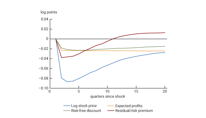
Figure 4 shows how the components of stock prices respond to a monetary policy shock thus identified. The experiment is one in which, starting from the steady state of the VAR, the economy receives a shock sufficient to raise the five-year Treasury yield by 25 basis points on impact. Such a shock causes one-year Treasury yields to rise by 31 basis points and 30-year yields to rise by 8 basis points in the period when it occurs. As shown by the blue line in figure 4, it causes a contemporaneous decline in stock prices of 0.08 log points. Based on the changes in Treasury yields and stock prices, as well as on the change in the expected path of corporate profits, one can calculate the three components of equity returns in equation 3 in each period after the shock.
4. Response of stock price components to monetary policy shock
Sources: Author’s calculations based on data from the U.S. Bureau of Economic Analysis, National Income and Product Accounts of the United States, and FT Wilshire 5000 Index from the Federal Reserve Bank of St. Louis, FRED; and Gürkaynak, Sack, and Wright (2007).
The initial decline in stock prices is split roughly equally between the three components, as shown in figure 4. Over time, the expected profits component stays nearly constant (since changes in expected cash flows at any given horizon are unforecastable). It seems unlikely that monetary policy has sizable permanent effects on real activity, so presumably its permanent effect on nominal profits derives mostly from its disinflationary effects. Meanwhile, the risk-free discounting component and the risk premium component of stock prices both return gradually to zero over time, as policy rates revert to the steady state. These transitory movements in discounting induce predictability in stock returns. In the long run, the expected change in stock prices is equal to the expected change in profits—a feature that is imposed by the error-correction structure of the model and one that is also consistent with the stationarity of both Treasury yields and the ERP.
Counterfactual simulation
I follow Gertler and Karadi (2015) and others by taking a medium-term Treasury bond yield—in this case, the five-year yield—to be the indicator of the monetary policy stance. The five-year yield has a correlation of 93% or higher with all other Treasury yields across the curve. It is affected significantly by changes in the contemporaneous federal funds target rate, expectations for the medium-term path of that rate (such as those that might result from forward guidance), and term premiums that can be affected by large-scale asset purchases (see note 3) or changes in rate volatility. Consequently, unlike very short-term or very long-term rates, it is likely to capture the effects of the full array of monetary policy tools.10
Based on the results of the structural identification, I calculate the series of quarterly monetary policy shocks that would have been sufficient to keep the five-year yield at the February 2020 level throughout the Covid period I study. The red lines in figures 2 and 3 show the paths of the Treasury yields and the stock market in the counterfactual scenario where these shocks are applied.11 By assumption, the counterfactual five-year Treasury yield is flat at a value of 1.33%. Given the multipliers on policy shocks, the counterfactual one-year Treasury yield hovers near its February 2020 value of 1.45% for a few quarters and then declines in order to be consistent with the flat five-year path. Thus, the scenario imagines a monetary policy that lowered short-term rates somewhat, though not as dramatically as was actually observed, while keeping the middle of the yield curve approximately stable around its initial value. In contrast, the counterfactual path for the 30-year Treasury yield is not much different from the actual path, reflecting the fact that the estimated multipliers on monetary shocks are relatively small at the long end. Thus, the model attributes most of the observed movements in long-term yields to nonmonetary factors, consistent with the intuition that monetary policy has only transitory effects.
The red line in figure 3 shows the model-implied counterfactual path taken by the stock market during this period. If policy had held the five-year Treasury yield at 1.33%, rather than allowing it to fall as low as 0.30% as it did in reality, the model implies that the stock market would have fallen by 34% on net over the first quarter of 2020—more than twice the decline actually observed. Moreover, under this scenario stocks would have only very gradually recovered and not exceeded their December 2019 value until 2022. In contrast, in the first quarter of 2022, the effects of monetary policy tightening, including expectations about increases in short-term interest rates and balance-sheet run-off that were yet to come, exerted a negative effect on the market.12 By the end of the sample, the observed value is about 15% below the counterfactual value.
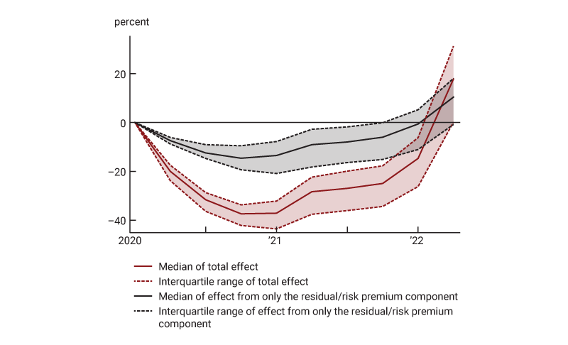
Looked at another way, the red line in figure 5 shows the proportion by which model-implied counterfactual stock prices fell short of the observed values (the percentage difference between the blue and red lines in figure 3)—a measure of the size of support that policy easing during the pandemic was providing to the stock market. The figure shows that at the peak of this support in late 2020, this difference was about 0.37%; in other words, policy was boosting prices by about $\frac{0.37}{1-0.37}$=59% from the level they would otherwise have had.
5. Effect of monetary policy on stock prices
Sources: Author’s calculations based on data from the U.S. Bureau of Economic Analysis, National Income and Product Accounts of the United States, and FT Wilshire 5000 Index from the Federal Reserve Bank of St. Louis, FRED; and Gürkaynak, Sack, and Wright (2007).
Using the counterfactual paths of Treasury yields, stock prices, and corporate profits, I recompute the decomposition presented earlier. I infer the entire Treasury yield curve, which is required for this decomposition, by first projecting the levels of yields, using all data from 1990 through 2022, onto the three yields that are included in the VAR. I then use the resulting factor loadings to compute complete quarter-by-quarter yield curves that are consistent with the counterfactual simulation. (As is well known, three factors are sufficient to explain nearly all of the variation in the yield curve—98% or more across all maturities, in this case—so this procedure involves very little loss of accuracy.) Figure 6 presents the results, reported as the difference between the components of stock returns in reality and under the counterfactual scenario. The numbers in this figure can be read as reflecting the effects of the monetary policy actions that occurred relative to what would have happened if medium-term interest rates had been held constant throughout the period.
6. Estimated effects of monetary policy on stock returns during Covid period
| Decomposition of policy effects on stock returns | ||||
|---|---|---|---|---|
| Time period | Effects of monetary policy on log stock price | Expected nominal profits | Risk-free discounting | Residual/risk premium |
| Initial shock and policy response December 2019–March 2020 |
+0.22 [0.19, 0.27] |
+0.09 [0.07, 0.12] |
+0.06 [0.05, 0.08] |
+0.08 [0.06, 0.09] |
| Rebound March–September 2020 |
+0.24 [0.19, 0.31] |
+0.09 [0.06, 0.12] |
+0.07 [0.05, 0.10] |
+0.08 [0.03, 0.14] |
| Continuing recovery September 2020–December 2021 |
–0.29 [–0.40, –0.17] |
–0.08 [–0.13, –0.05] |
–0.08 [–0.12, –0.05] |
–0.11 [–0.21, –0.05] |
| Beginning of policy tightening December 2021–March 2022 |
–0.32 [–0.37, –0.27] |
–0.11 [–0.15, –0.09] |
–0.09 [–0.11, –0.07] |
–0.11 [–0.14, –0.08] |
According to the model, monetary policy affected stock prices roughly equally through all three channels throughout the Covid era. During the first three quarters of the pandemic (summing the top two rows of figure 6), expected profits, risk-free discounting, and risk premiums contributed 0.18, 0.13, and 0.16 log points to stock prices, respectively. Between the third quarter of 2020 and the fourth quarter of 2021, policy rates remained low, but anticipated tightening gradually led to a rise in the five-year Treasury yield, pushing stock prices 0.29 log points lower than they otherwise would have been. The largest effect was through risk premiums, but profits and discounting also contributed substantially. As policy rates began rising, large-scale asset purchases ended, and market participants priced in a faster pace of tightening, these effects continued, again spread across all three components.
The risk-free discounting effects on stock prices are to be expected of monetary policy, and the effects on nominal profits are intuitive given monetary policy’s impact on both real activity and prices; however, the response of the risk premium component is perhaps surprising. The black line in figure 5 shows the amount of support that the model indicates monetary policy would have provided to the stock market if it had operated through this component alone. Looked at in this way, fluctuations in risk premiums accounted for more than one-third of monetary policy’s overall effect on the stock market through the end of 2020. Likewise, when policy began to subtract from equity prices in 2022, the risk premium component was the primary culprit. Again, I should note that there is some reason to take this conclusion with a grain of salt, since misspecification in the VAR model as a measure of market expectations would show up in the “risk premium” component. Even so, the results are consistent with recent literature that ascribes a significant role to the risk-taking channel (see, for example, Bauer, Bernanke, and Milstein, 2023).
Conclusion
In this article, I analyzed the behavior of the stock market during the two years following the onset of the Covid-19 pandemic by decomposing equity price movements into changes in three components: expected cash flows, risk-free rates, and a residual component containing risk premiums. The stock market is important as a source of wealth for consumers, a source of financing for firms, a source of information for policymakers, and a source of interest for researchers. The analysis shows that the early decline in equity prices resulted mainly from the residual component, consistent with a large swing in the equity risk premium, while the subsequent rally was due to both a recovery in the equity risk premium and higher expectations for corporate profits. Meanwhile, the decline and rebound of the U.S. Treasury yield curve pushed against this tide, keeping stock prices somewhat higher than they otherwise would have been in early 2020 and somewhat lower in early 2022. Monetary policy helped prevent a much bigger catastrophe in stock prices; the model estimates that without this support, equities would have been 37% lower at their trough. Policy worked through all three components of stock prices. Among other implications, the results suggest that monetary policy’s effects on risk premiums could be considered as a potentially key transmission channel in both empirical analyses and theoretical treatments of monetary policy.
Notes
1 Board of Governors of the Federal Reserve System (2022, p. 44).
2 The risk-taking channel refers to various mechanisms by which lower interest rates may induce financial institutions to take on additional risk. See, for example, Borio and Zhu (2012), Morris and Shin (2016), and Bauer, Bernanke, and Milstein (2023).
3 Specifically, these purchases are large-scale purchases of U.S. Treasury securities and mortgage-backed securities issued by government-sponsored enterprises and federal agencies that the Federal Reserve has made to help achieve its monetary policy objectives (see, for instance, note 1). Also referred to as quantitative easing, or QE, these large-scale asset purchases are typically used to provide additional monetary stimulus when the target federal funds rate—the Fed’s traditional policy tool for changing the short-term nominal interest rate—has already been reduced to near zero. For an analysis on the benefits and costs of large-scale asset purchases, see Carlson et al. (2020).
4 If $M_{t}^{\left( n \right)}$ is the stochastic discount factor for cash flows n periods hence, then under no-arbitrage conditions, stock prices are given by \[{\text{exp}} \left[ {{s}_{t}} \right]=\sum\limits_{n}{{{\text{E}}_{t}}\left[ M_{t}^{(n)}{{\prod }_{t+n}} \right]}=\sum\limits_{n}{{{\text{E}}_{t}}}\left[ M_{t}^{(n)} \right]{{\text{E}}_{t}}\left[ {{\prod }_{t+n}} \right]+\sum\limits_{n}{{{\text{cov}}_{t}}\left[ M_{t}^{(n)},{{\prod }_{t+n}} \right]}={{V}_{t}}+\sum\limits_{n}{{{\text{cov}}_{t}}\left[ M_{t}^{(n)},{{\prod }_{t+n}} \right]},\] since ${{\text{E}}_{t}}\left[ M_{t}^{(n)} \right]= \unicode{x03B4} _{t}^{(n)}.$ Consequently, one can write ${{ERP}_{t}}=\log \left( {1+{{\sum }_{n}}{{\text{cov}}_{t}}\left[ M_{t}^{(n)},{{\prod }_{t+n}} \right]}/{{{V}_{t}}}\right),$ consistent with the intuition that greater co-movement between cash flows and discount factors should require higher expected returns and thus lower asset prices.
5 Adding inflation to the model could provide some interesting further insights into the sources of cash-flow and discount-rate variation, but it is not necessary for the decomposition presented here.
6 Another caveat is that, as will all time-series modeling with fixed parameters, changes in the structural environment could shift the reduced-form parameters. This could be a particular concern during the period in question, which saw many unprecedented economic developments.
7 Beyond the 30-year maturity, where data are not available, I assume that yields converge at a constant rate across maturities from 30-year spot rates to their infinite-horizon level, which is taken to be the steady-state value of y(30).
8 Bauer and Swanson (2023) have recently argued that the empirical patterns that Nakamura and Steinsson (2018) interpret as a Fed information effect actually reflect changing market perceptions of the Fed’s reaction function associated with policy surprises. My identification restrictions also exclude this type of contaminating factor.
9 Following D’Amico and King (2023b), I also impose that the expected short-term rate moves in the opposite direction of expected economic activity (profits, in this case) for at least four quarters following a shock. This restriction is largely redundant, given the sign restriction on the risk-free discount term, and the results are robust to its removal.
10 That said, the results in this section also generally hold if one-year Treasury yields are used as the measure of policy.
11 All estimates reported for the counterfactual simulation are based on the medians of the posterior distributions. To measure statistical uncertainty, I report interquartile ranges of the posteriors (that is, the middle 50% of the distribution).
12 D’Amico and King (2023a) discuss how expectations for eventual policy tightening exerted restraint on the economy even before the FOMC had significantly raised policy rates.
Appendix: Estimation and Identification Details
Let xt be a vector containing, in order, one-year, five-year, and 30-year zero-coupon U.S. Treasury yields; the log change in nominal corporate profits; the log change in the stock market index; and the difference between the log levels of profits and stock prices (the “error correction” term). The vector autoregression is specified as
\[\textbf{x}_{t+1} = \textbf{a} + \textbf{Ax}_{t} + \textbf{e}_{t}.\]
(Information criteria suggest a lag length of 1 is optimal.) This model is estimated by Bayesian methods, assuming a flat prior for the coefficients and, for the sake of simplicity, treating the covariance matrix of et , S, as given.
The unconditional mean of xt is given by
\[\bar{\textbf{x}}=\textbf{a}{{\left( \textbf{I}-\textbf{A} \right)}^{-1}}.\]
I sample draws j from the posterior distribution of the VAR parameters, rejecting draws for which ${{\bar{\textbf{x}}}_{\left\{ 3 \right\},\,j}}$ (the mean of the 30-year yield) is less than ${{\bar{\textbf{x}}}_{\left\{ 4 \right\},\,j}}$ (the mean of profit growth). This ensures that the risk-free discounted value of profits exist. (I also reject any draw for which the VAR violates the conditions for stationarity.) Sampling continues until 1,000 draws are kept.
For each accepted draw of the estimated reduced-form VAR parameters, the structural identification of the monetary-policy shocks proceeds as follows.
1. Draw a sequence of matrices Mi such that, for each draw $i,{\textbf{M}_i}{\textbf{M}^{′}_{i}}={\textbf{S}}$ Designate the first row of Mi as mi. This will be the vector of candidate multipliers on the monetary policy shock. Rotate Mi such that m{2},i , the element corresponding to the contemporaneous effect of this shock on the five-year yield, is positive.
2. For each draw, calculate the VAR-implied response to an impulse of magnitude mi over 800 quarters. This is given by $\textbf{A}_{j}^{h}{{\textbf{m}}_{i}},$ where h = 0, ..., 800 is the matrix power.
3. From the impulse response for profits, calculate the term $T_{i}^{1}=\sum{_{n=1}^{\infty }}\unicode{x03B4} _{0}^{(n)}\left( {{\text{E}}_{1}}\left[ {{\prod }_{n-1}} \right]-{{\text{E}}_{0}}\left[ {{\prod }_{n-1}} \right] \right)$ using steady-state discount factors for $\unicode{x03B4} _{0}^{^{(n)}}.$ (The latter are calculated using ${{\bar{\textbf{x}}}_{\left\{ 1 \right\},\,j}}$ through ${{\bar{\textbf{x}}}_{\left\{ 3 \right\},\,j}}$ and applying the estimated yield curve loadings to derive the entire curve). This term reflects the impact of a shock on the expected-profits component of stock prices.
4. From the impulse response for yields, calculate the term $T_{i}^{2}=\sum{_{n=1}^{\infty }}\unicode{x0394} \unicode{x03B4} _{1}^{(n)}{{\text{E}}_{0}}\left[ {{\prod }_{n}} \right],$ where ${{\text{E}}_{0}}\left[ {{\prod }_{n}} \right]$ is calculated based on the steady-state growth rate of profits ${{\bar{\textbf{x}}}_{\left\{ 4 \right\},\,j}}.$ This term reflects the impact of a shock on the risk-free discount component of stock prices.
5. Calculate the component of the initial stock price response not accounted for by either of the other two terms, $T_{i}^{3}={{\textbf{m}}_{i}}_{,\left\{ 5 \right\}}-T_{i}^{1}-T_{i}^{2}.$ This term reflects the equity risk premium.
6. Reject the draw if $T_{i}^{1}\text{, }T_{i}^{2}\text{, or}\,\,T_{i}^{3}$ is positive or if ${{\left( \textbf{A}_{j}^{4}{{\textbf{m}}_{i}} \right)}_{\left\{ 1 \right\}}}$ is negative.
Sampling continues until 1,000 draws mi are kept for each draw j. I find the “median target” draw mMTj by computing the Euclidean distance from each draw to the vector median of mi. I keep this vector as the contemporaneous multipliers associated with the VAR-parameter draw j. The collection of these vectors constitutes the posterior distribution of the multipliers on the monetary policy shocks.
References
Bauer, Michael D., Ben S. Bernanke, and Eric Milstein, 2023, “Risk appetite and the risk-taking channel of monetary policy,” Journal of Economic Perspectives, Vol. 37, No. 1, Winter, pp. 77–100. Crossref
Bauer, Michael D., and Eric T. Swanson, 2023, “An alternative explanation for the ‘Fed information effect,’” American Economic Review, Vol. 113, No. 3, March, pp. 664–700. Crossref
Bekaert, Geert, Marie Hoerova, and Marco Lo Duca, 2013, “Risk, uncertainty and monetary policy,” Journal of Monetary Economics, Vol. 60, No. 7, October, pp. 771–788. Crossref
Bernanke, Ben S., and Kenneth N. Kuttner, 2005, “What explains the stock market’s reaction to Federal Reserve policy?,” Journal of Finance, Vol. 60, No. 3, June, pp. 1221–1257. Crossref
Board of Governors of the Federal Reserve System, 2022, Monetary Policy Report, Washington, DC, February 25, available online.
Borio, Claudio, and Haibin Zhu, 2012, “Capital regulation, risk-taking and monetary policy: A missing link in the transmission mechanism?,” Journal of Financial Stability, Vol. 8, No. 4, December, pp. 236–251. Crossref
Campbell, John Y., and Robert J. Shiller, 1988a, “Stock prices, earnings, and expected dividends,” Journal of Finance, Vol. 43, No. 3, July, pp. 661–676. Crossref
Campbell, John Y., and Robert J. Shiller, 1988b, “The dividend-price ratio and expectations of future dividends and discount factors,” Review of Financial Studies, Vol. 1, No. 3, July, pp. 195–228. Crossref
Carlson, Mark, Stefania D’Amico, Cristina Fuentes-Albero, Bernd Schlusche, and Paul Wood, 2020, “Issues in the use of the balance sheet tool,” Finance and Economics Discussion Series, Board of Governors of the Federal Reserve System, No. 2020-071, August. Crossref
Cieslak, Anna, and Hao Pang, 2021, “Common shocks in stocks and bonds,” Journal of Financial Economics, Vol. 142, No. 2, November, pp. 880–904. Crossref
Cox, Josue, Daniel L. Greenwald, and Sydney C. Ludvigson, 2020, “What explains the COVID-19 stock market?,” National Bureau of Economic Research, working paper, No. 27784, September. Crossref
D’Amico, Stefania, and Thomas B. King, 2023a, “Past and future effects of the recent monetary policy tightening,” Chicago Fed Letter, Federal Reserve Bank of Chicago, No. 483, September. Crossref
D’Amico, Stefania, and Thomas B. King, 2023b, “What does anticipated monetary policy do?,” Journal of Monetary Economics, Vol. 138, September, pp. 123–139. Crossref
D’Amico, Stefania, Thomas B. King, and Min Wei, 2016, “Macroeconomic sources of recent interest rate fluctuations,” Chicago Fed Letter, Federal Reserve Bank of Chicago, No. 363, available online.
Fry, Renée, and Adrian Pagan, 2011, “Sign restrictions in structural vector autoregressions: A critical review,” Journal of Economic Literature, Vol. 49, No. 4, December, pp. 938–960. Crossref
Gertler, Mark, and Peter Karadi, 2015, “Monetary surprises, credit costs, and economic activity,” American Economic Journal: Macroeconomics, Vol. 7, No. 1, January, pp. 44–76. Crossref
Gormsen, Niels Joachim, and Ralph S. J. Koijen, 2020, “Coronavirus: Impact on stock prices and growth expectations,” Review of Asset Pricing Studies, Vol. 10, No. 4, December, pp. 574–597. Crossref
Gürkaynak, Refet S., Brian Sack, and Eric T. Swanson, 2005, “Do actions speak louder than words? The response of asset prices to monetary policy actions and statements,” International Journal of Central Banking, Vol. 1, No. 1, May, pp. 55–93, available online.
Gürkaynak, Refet S., Brian Sack, and Jonathan H. Wright, 2007, “The U.S. Treasury yield curve: 1961 to the present,” Journal of Monetary Economics, Vol. 54, No. 8, November, pp. 2291–2304. Crossref
Jarociński, Marek, and Peter Karadi, 2020, “Deconstructing monetary policy surprises—The role of information shocks,” American Economic Journal: Macroeconomics, Vol. 12, No. 2, April, pp. 1–43. Crossref
Knox, Benjamin, and Annette Vissing-Jorgensen, 2022, “A stock return decomposition using observables,” Finance and Economics Discussion Series, Board of Governors of the Federal Reserve System, No. 2022-014, March. Crossref
Landier, Augustin, and David Thesmar, 2020, “Earnings expectations during the COVID-19 crisis,” Review of Asset Pricing Studies, Vol. 10, No. 4, December, pp. 598–617. Crossref
Matheson, Troy, and Emil Stavrev, 2014, “News and monetary shocks at a high frequency: A simple approach,” Economics Letters, Vol. 125, No. 2, November, pp. 282–286. Crossref
Morris, Stephen, and Hyun Song Shin, 2016, “Risk premium shifts in monetary policy: A coordination approach,” in Monetary Policy Through Asset Markets: Lessons from Unconventional Measures and Implications for an Integrated World, Elías Albagli, Diego Saravia, and Michael Woodford (eds.), Santiago, Chile: Central Bank of Chile, pp. 131–150.
Nakamura, Emi, and Jón Steinsson, 2018, “High-frequency identification of monetary non-neutrality: The information effect,” Quarterly Journal of Economics, Vol. 133, No. 3, August, pp. 1283–1330. Crossref
Rigobon, Roberto, and Brian Sack, 2004, “The impact of monetary policy on asset prices,” Journal of Monetary Economics, Vol. 51, No. 8, November, pp. 1553–1575. Crossref


