

We offer a method to derive a risk-premium adjustment to the risk-neutral policy rate path implied by raw financial quotes. Our method aims to preserve the information derived from high-frequency data, while also filtering out noise unrelated to future macro-finance conditions.
When we talk about the policy rate path, we are referring to the expected trajectory of the federal funds rate (FFR). Several approaches can be used to gauge expectations about the path of the FFR. One of the most common is to use quotes on interest rate derivatives, such as overnight indexed swaps (OIS) and FFR futures. This method is appealing because it provides readings on policy rate expectations at a very high frequency. Researchers can use this to understand how market expectations change following specific monetary policy events, such as Federal Open Market Committee (FOMC) meetings, Fed officials’ speeches and testimonies before congressional committees, and releases of FOMC meeting minutes.
To correctly extract expectations about the policy rate path from quotes on interest rate derivatives, we need to distinguish the “true” expectations from the risk premium. This distinction allows us to understand better how each of the two components changes as a result of monetary policy communications. We offer a method to estimate FFR risk premiums to adjust the risk-neutral policy rate path implied by raw financial quotes. Our method aims to preserve the information derived from high-frequency data, as in Priebsch (2017), while exploiting the no-arbitrage equilibrium condition implied by macro-finance models, as done in Diercks and Carl (2019). This second feature should help filter out risk-premium adjustments unrelated to macro-finance conditions.
To understand the potential relevance of the risk-premium adjustment, figure 1 plots a rough proxy of the six- and 12-month FFR risk premium,1 which is the difference between OIS rates and Blue Chip Financial Forecasts (BCFF) of the FFR at six- and 12-month horizons. Survey forecasts like the BCFF should not be contaminated by financial risk premiums; as a result, their divergence from market-based expectations like OIS rates hints at the existence of risk premiums in those measures of expectations.2 This proxy suggests that the per-month risk premium could be sizable, time-varying, and changing in sign due to variations in investor risk assessment. Hence, it could significantly alter the expected policy rate path and, if ignored, could lead to a misrepresentation of the perceived stance of monetary policy and its fluctuations in response to monetary policy decisions.
1. Difference between OIS and survey forecasts of FFR
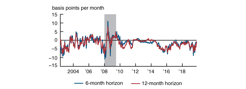
Sources: Authors’ calculations based on data from Blue Chip Financial Forecasts, Bloomberg Financial LP, and D’Amico, Kim, and Wei (2018).
Although the difference between OIS rates and BCFF of the FFR serves as a good starting point for the estimation of risk premiums, more can be done to filter out noise and derive a measure of the risk-premium adjustment that is more closely related to macroeconomic risk factors, such as inflation risk and real-growth risk.
Methodology
Our method, similar to that of Diercks and Carl (2019), starts with the standard no-arbitrage condition common to many macro-finance models:
1) $R{{P}_{t\text{ }+\text{ }h}}\approx -\text{Co}{{\text{v}}_{t}}\left( {{M}_{t\text{ }+\text{ }h}},\text{ }{{N}_{t\text{ }+\text{ }h}} \right),~$
where $RP$ denotes the risk premium, $h$ the time horizon, $N$ a nominal interest rate, and $M$ denotes the stochastic discount factor (SDF).3 This condition indicates that the sign and size of the RP on a nominal rate, at a given horizon, depends on the co-movement between the SDF and the nominal rate over the same horizon, which usually reflects the length of the investment period.The SDF is driven by the growth rate of investors’ marginal utility of consumption or wealth. If investor wealth is expected to decrease at time $t+h$ (implying a bad state of the economy), then the SDF will be high at time $t$ as investors will value future changes in wealth more than current changes in wealth. This implies that if an asset’s cash flows are expected to decrease when the SDF is increasing (i.e., a negative covariance in equation 1), then the $RP$ will be positive, as investors will require a higher return to hold a riskier asset. In contrast, if an asset’s cash flows are expected to increase when the SDF is increasing (i.e., a positive covariance in equation 1) the $RP$ will be negative, and the asset will be viewed as having very good hedging properties as investors will be willing to receive a lower return to hold a safer asset.
The covariance between the SDF and the nominal interest rate is difficult to measure. It is often approximated by the co-movements between low-frequency macro variables. For example, Diercks and Carl (2019) use various monthly measures of inflation and real activity.4 In our approach, we approximate this covariance with the co-movements between measures of expected growth and inflation implied by financial variables. This helps us to obtain high-frequency estimates of the $RP$ and exploit the information contained in forward-looking variables.
We can break apart the covariance in equation 1 into two components with the insight of Nakata and Tanaka (2016):
2) $R{{P}_{t\text{ }+\text{ }h}}\approx -[\text{Co}{{\text{v}}_{t}}\left( {{M}_{t\text{ }+\text{ }h}},\text{ }{{\pi }_{t\text{ }+\text{ }h}} \right)\text{ }+\text{ Co}{{\text{v}}_{t}}\left( {{M}_{t\text{ }+\text{ }h}},\text{ }{{R}_{t\text{ }+\text{ }h}} \right)]$,
where $\pi $ denotes the inflation rate and $R$ a real rate. In equation 2, the first covariance captures the component of the $RP$ related to inflation risk, and the second covariance captures the component of the $RP$ related to real-growth risk.To approximate each covariance in equation 2, we follow the methodology of Gourio and Ngo (2020). We approximate the first covariance with the rolling correlation between changes in stock prices (SP), a proxy for expected growth, and changes in inflation compensation implied by Treasury Inflation-Protected Securities (TIPS), a proxy for expected inflation. We approximate the second covariance with the rolling correlation between changes in stock prices and changes in the expected real rate implied by TIPS, a proxy for the expected real rate.5 Using TIPS limits the length of our sample period, which is a shortcoming of our methodology.
Combining the rough proxy of the $RP$ described in figure 1 with the methodology detailed in equation 2, we can estimate the following relation by ordinary least squares (OLS) at the weekly frequency from May 2002 to the week ending on November 1, 2019:
3) $OI{{S}_{t+h}}-E_{t}^{BCFF}\left( FF{{R}_{t+h}} \right)=\alpha +{{\beta }_{1}}\left[ -\text{Cor}{{\text{r}}_{t}}\left( \Delta S{{P}_{t+h,}}\Delta \pi _{t+h}^{TIPS} \right) \right]+{{\beta }_{2}}\left[ -\text{Cor}{{\text{r}}_{t}}\left( \Delta S{{P}_{t+h,}}\,\Delta R_{\,t+h}^{TIPS} \right) \right]+{{\varepsilon }_{t}},$
where the dependent variable is the same as in figure 1, the difference between OIS rates and the BCFF of the FFR; the change in stock prices, $\Delta SP,$ is measured by the log returns of the S&P 500 Index; and both changes in expected inflation, $\Delta {{\pi }^{TIPS}},$ and the expected real rate,$\Delta {{R}^{TIPS}},$ are derived from the dynamic term-structure model of D’Amico, Kim, and Wei (2018). Their model helps avoid the liquidity issues affecting TIPS and therefore allows us to compute changes in expected inflation and real rates that are unrelated to changes in the broad liquidity of the TIPS market. Finally, we estimate our model at various horizons up to 15 months, matching the maturity of the dependent variable to the maturities of the independent variables used in the covariance approximation.
Results
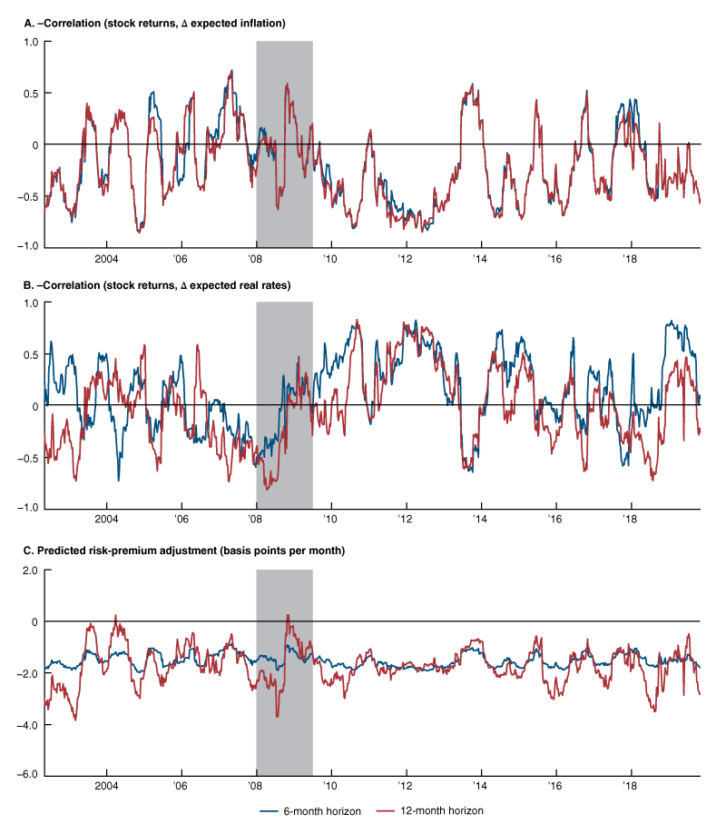
Our estimate of the risk-premium adjustment is the predicted component of the OLS regression at each horizon. The adjustment and both correlations’ components are shown in figure 2 for the six- and 12-month horizons, and the estimated coefficients $\alpha ,\text{ }{{\beta }_{1}},\text{ and }{{\beta }_{2}}$ are shown in box 1 at the three-, six-, nine-, 12-, and 15-month horizons. The estimated value for the constant in the OLS regression is negative at all horizons, which is not surprising considering that in our sample period the dependent variable is almost always negative (figure 1). In contrast, the estimates for ${{\beta }_{1}}$ and ${{\beta }_{2}}$ are almost always positive; their magnitude increases with the horizon. At each horizon, ${{\beta }_{1}}$ tends to be larger than ${{\beta }_{2}},$ which suggests that the inflation risk might be more relevant for the risk-premium adjustment.
As shown in figure 2, similar to Priebsch (2017), our risk-premium adjustment displays significant time variation, and post-2004 it is almost always negative, averaging about –1.5 and –1.6 basis points per month at the six- and 12-month horizons, respectively. This implies that in our sample period, the unadjusted market-based policy path is almost always lower than the “true” expected policy path implied by our risk-premium adjustment. However, the difference between the unadjusted and adjusted market-based policy paths is often not as large as figure 1 suggests. This is because the correlations used in equation 3, which capture the main macro-finance risk factors, likely help filter out parts of the nonfundamental noise.
2. Components and output of equation 3
As previously mentioned, the main disadvantage of our model is that due to the TIPS data starting later than our other data sources, our sample period is shorter than those used in other studies. Therefore, our model is not estimated during periods in which the predicted risk premium on the FFR tends to be positive, as for example in the longer sample period of Diercks and Carl (2019) and Priebsch (2017), which estimate risk premiums starting in the early 1990s.
Our method has four distinct advantages over existing methods. First, it uses rolling correlations in an OLS regression, which is computationally simpler than previous studies. Second, it substitutes macroeconomic variables, which are backward-looking in nature, with financial variables, which contain information about future expected real rate and inflation. Third, it employs only market-based macroeconomic information, preserving the high frequency of interest rate derivatives, giving us a better sense of when changes in policy expectations and risk perceptions are happening. Finally, the two-correlation structure better isolates how fluctuations in inflation risk and real-growth risk affect changes in the risk premium.
Case study
As an example of this adjustment, we focus on the period of October–November 2019. From the panels A and B of figure 2, it is evident that both proxies for the real and inflation risk factors have been declining sharply, with the inflation risk moving further into negative territory.6 This potentially reflects the FOMC’s concerns about inflation still running below 2% and market-based measures of inflation compensation being low.7 Further, on October 31, 2019, news that Chinese officials expressed doubts over the prospects of reaching a longer-term comprehensive trade agreement with the U.S. might have contributed to the latest decline in the real risk factor. These developments translated to a predicted risk-premium adjustment of about –2 and –3 basis points per month at the six- and 12-month horizons, respectively. This suggests that investors consider short-term nominal assets a good hedge as they expect real rates, inflation, and stock returns to decline in the near term.
As shown in figure 3, these risk-premium adjustments result in a “true” expected policy rate path (green line) well above the unadjusted policy rate path implied by the raw OIS quotes (blue line). Interestingly, the adjusted policy rate path seems more consistent with the suite of communications of the October 2019 FOMC, which have reportedly been viewed as suggesting that further reductions in the target range were less likely, consistent with a near-term pause. Finally, it is worth noticing that the adjusted policy rate path is also above the survey-based path, likely in part because the BCFF survey information does not reflect communications released at the October 2019 FOMC meeting.8
3. Adjusted versus unadjusted policy rate path, week of October 28 to November 1, 2019
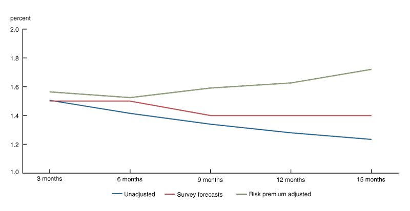
This example provides one of the many instances in which the risk-premium adjustment implies an expected policy rate path well above the unadjusted market-based path, suggesting that accounting for the risk premium can lead to a markedly different interpretation of the perceived stance of monetary policy. Therefore, we argue that our methodology, due to the advantages listed above, is a necessary supplement to the existing frameworks in the literature.
Box 1. Coefficient estimates
| $\alpha$ | $\beta_{1}$ | $\beta_{2}$ | |
|---|---|---|---|
| 3 months | –0.054*** | 0.006 | –0.003 |
| 6 months | –0.083*** | 0.049** | 0.012 |
| 9 months | –1.118*** | 0.209*** | 0.188*** |
| 12 months | –0.139*** | 0.285*** | 0.206*** |
| 15 months | –0.190*** | 0.360*** | 0.298*** |
Sources: Authors’ calculations based on data from Blue Chip Financial Forecasts, Bloomberg Financial LP, and D’Amico, Kim, and Wei (2018).
Notes
1 The maturity of the risk-premium adjustment depends on the expiration of the underlying interest rate derivatives and the horizon of the survey forecasts, which are closely matched here.
2 However, survey forecasts can reflect other subjective biases that cause them to deviate from the “true” expectations.
3 The stochastic discount factor (SDF) is approximately equal to the log of the ratio of the marginal utility at time $t+h$ and the marginal utility at time $t.$
4 For inflation measures, they use data such as CPI-U and PCE-All. For real activity measures, they use the 12-month percentage change in industrial production and 12-month percentage change in nonfarm payrolls.
5 Correlations are computed over 16-week rolling windows for each horizon.
6 Based on equation 1, a decline in the proxies for the macro-finance risk factors corresponds to the correlations becoming more positive and in turn a negative risk premium.
7 See, for example, the FOMC statements of July, September, and October 2019, available online.
8 This is because the participants of the November 1 BCFF submit their survey results up to a week prior.
References
D’Amico, Stefania, Don H. Kim, and Min Wei, 2018, “Tips from TIPS: The informational content of Treasury Inflation-Protected Security prices,” Journal of Financial and Quantitative Analysis, Vol. 53, No. 1, February, pp. 395–436. Crossref
Diercks, Anthony, and Uri Carl, 2019, “A simple macro-finance measure of risk premia in fed funds futures,” FEDS Notes, Board of Governors of the Federal Reserve System, January 8. Crossref
Gourio, François, and Phuong Ngo, 2020, “Risk premia at the ZLB: A macroeconomic interpretation,” Cleveland State University, working paper, January 2, available online.
Nakata, Taisuke, and Hiroatsu Tanaka, 2016, “Equilibrium yield curves and the interest rate lower bound,” Finance and Economics Discussion Series, Board of Governors of the Federal Reserve System, No. 2016-085, October. Crossref
Priebsch, Marcel, 2017, “A shadow rate model of intermediate-term policy rate expectations,” FEDS Notes, Board of Governors of the Federal Reserve System, October 4. Crossref


