

Dedicatory remarks
On November 10, 2020, I delivered the Alejandro Justiniano Keynote Lecture at the Macroeconomics System Committee Meeting of the Federal Reserve. This lecture series, dedicated to my Chicago Fed colleague who passed away prematurely in 2018, showcases policy-relevant research by economists from the Federal Reserve System. This article is adapted from that presentation. Alejandro did not work with theoretical models of bubbles, although he did write several influential papers on the U.S. housing boom of the mid-2000s that many believe was a bubble. Rather than discuss topics that directly relate to Alejandro’s research, my lecture took its inspiration from the way Alejandro advocated for (and practiced) using research to inform macroeconomic policy.
Introduction and summary
Policymakers have long debated how to respond to asset price booms—especially given the potential consequences if these booms give way to asset price collapses. Interest in this question has been reinforced by the fact that two asset booms in the United States around the turn of the millennium—the dot-com boom of the late 1990s and the housing boom of the mid-2000s—were associated with bad subsequent outcomes. In each case, the price of a broad class of assets—equity shares in technology firms in the earlier case and housing in the later one—increased at high rates before the price turned around and collapsed even more rapidly, erasing in a single year most of the price gains accrued in previous years. These price declines occurred either just before or concurrently with the onset of a recession as determined by the National Bureau of Economic Research’s (NBER) Business Cycle Dating Committee.1 Many observers view the timing of these recessions as more than coincidental, and regard these episodes as evidence of the potential harm that may be unleashed when asset prices are allowed to grow unchecked.
Assessing the desirability of intervening against asset booms requires a guiding framework to help determine when and why asset booms can occur and whether policy intervention might improve social welfare in such situations. In this article, I discuss one such framework based on models of asset bubbles, or situations in which assets trade at a price differing from—and, of particular interest, exceeding—the value of the underlying cash flows that the asset is expected to pay out. Inherent to this approach is the idea that during booms, asset prices rise to levels that are detached from what these assets are intrinsically worth. Models that can capture this phenomenon could help determine what policy response (if any) might be appropriate if asset booms are associated with excessively high asset prices. Even if it may be difficult in practice to determine the intrinsic value of an asset and gauge whether it is overvalued, a framework for evaluating which policies are appropriate when assets are overvalued can still be useful. Policymakers may have reason to believe assets are likely to be overvalued even if they cannot be entirely sure—if, for example, asset prices are extremely high and can only be justified by scenarios that are relatively unlikely. In those cases, a model can still suggest a general direction for policy given the policymakers’ concerns.
My discussion revolves around two main themes. First, I argue that models of bubbles seem like a natural framework for studying asset booms. Indeed, this is why I was drawn to working with these models in my own research. Second, as I allude to in the title of this article, recent work should make us question whether the concept of a bubble is indeed important for policymakers who want to know whether to intervene against an asset boom to forestall a possibly severe recession. This is because the logic that emerges from recent work that uses models of bubbles to explore this question reveals that whether the underlying asset is in fact a bubble may not matter; the same case for intervention during booms can be made when asset prices properly reflect fundamentals. In this sense, the focus on modeling asset booms as bubbles may have served as a distraction, encouraging policymakers to unnecessarily focus on the question of whether an asset is overvalued before acting during an asset boom.
To be clear, my point is not to argue against models of bubbles, either as thought exercises or as ways to think about particular episodes such as the dot-com boom in the late 1990s or the housing boom in the mid-2000s. To the contrary, the possibility of asset bubbles remains an important and intriguing phenomenon worth studying. The rise of cryptocurrencies that command high prices despite not paying any dividends serves as a reminder that assets can trade at prices not justified by their underlying fundamentals. The prospect of assets trading at prices not tied to these assets’ cash flows can have potentially important welfare consequences. On the one hand, as economist Jaume Ventura argues, creating wealth out of thin air at no cost is something society benefits from and should celebrate.2 On the other hand, letting assets trade above their true worth may encourage resource misallocation by providing agents with incentives to produce more assets that sell at a high price but generate little in the way of dividends that benefit society. Understanding why bubbles can occur remains an important goal for economic research and a pressing question for policymakers. The point of this article is narrower: It is only to argue that the focus on bubbles may have led to a misperception that identifying bubbles is a necessary step for policymakers who are contemplating acting against an asset boom because they anticipate a recession if and when the boom becomes a bust.
Digression on a financial stability mandate for central banks
Before turning to questions of when and how the concept of a bubble might be important, I want to relate my discussion to the broader policy debate prompted by the 2008 global financial crisis. Since the crisis, there have been growing calls for central banks to adopt an explicit financial stability mandate to supplement their existing mandates, such as price stability and maximum employment.3 The idea is for central banks to use both regulatory and monetary policy tools to promote the stability of the financial systems they oversee. A milder version of this approach argues that even without an explicit mandate to promote financial stability, central banks should take into account how financial stability considerations can impact inflation and employment, which they are already mandated to help stabilize.4 Interest either in an explicit financial stability mandate or in a proactive response to threats that financial imbalances may pose for inflation and output intensified after the experience of financial intermediaries during the global financial crisis. Since these intermediaries incurred losses from housing-related assets when house prices fell starting in 2007, one way that central banks could have promoted financial stability would have been to intervene back when house prices surged. In that sense, there is a natural connection between intervening against asset booms and designing policies that incorporate financial stability concerns in some way.
However, the two policy directives are not identical. While asset booms can be related to financial instability, the two phenomena do not always overlap. For example, during the dot-com boom of the late 1990s, the total extent of borrowing against equity shares in technology firms was fairly limited, and the collapse in the stock prices of dot-com firms had little effect on the financial system. Consistent with this, it is only after the subsequent global financial crisis that calls for a financial stability mandate intensified. Conversely, the U.S. savings and loans crisis of the early 1990s involved a rise in risky lending by financial intermediaries that led to stresses in the financial system, though not a rapid appreciation in the price of any particular asset class. In line with this distinction, several recent research papers such as Svensson (2017), Gourio, Kashyap, and Sim (2018), and Boissay et al. (2022) study financial crises without any reference to asset booms. Interventions against asset booms can matter for financial stability, but an imperative to act against booms is not the same as a mandate to ensure the stability of the financial system.
Historical examples of asset booms
The argument that policymakers should intervene against asset booms is typically motivated by prominent historical episodes in which a rapid surge in asset prices was associated with bad subsequent outcomes. I begin by reviewing some of these examples to provide a sense of the phenomenon that policymakers would want a model of asset booms to presumably capture.
As noted in the introduction and summary, the dot-com boom of the 1990s and the housing boom of the mid-2000s generated interest in interventions against asset booms. Figure 1 illustrates the first of these episodes. It shows the Nasdaq-100 index between 1995 and 2005.5 The Nasdaq Stock Market index is more heavily weighted toward technology firms than other major stock indexes in the United States and so better reflects the prices of such firms. The shaded region in the figure corresponds to the recession as identified by the NBER. As evident in the figure, the Nasdaq-100 index increased more than fourfold between January 1999 and March 2000. It then fell to a third of its peak value over the next 12 months—just before March 2001, when a recession began according to the NBER. All of the gains between January 1999 and the peak were erased by November 2001, which marked the end of the recession as declared by the NBER.
Figure 1. Nasdaq-100, January 1995–December 2005
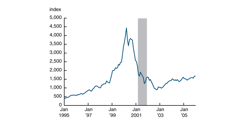
Source: Nasdaq Inc. from the Federal Reserve Bank of St. Louis, FRED (Federal Reserve Economic Data).
The housing boom of the mid-2000s that occurred only a few years later played out similarly in certain key respects. Figure 2 illustrates the Case-Shiller home price indexes for the United States as a whole and for Phoenix and Las Vegas—the two cities that experienced the fastest rates of four-quarter house price appreciation between the first quarter of 2000 and when city-specific house prices peaked.6 For the nation as a whole, house prices rose 85 percent between 2000 and 2006. In Las Vegas and Phoenix, house prices rose even more dramatically, essentially doubling between 2004 and 2006. House prices, both overall and in these cities, leveled off in 2006 and started falling in 2007. House prices then precipitously fell in 2008, coinciding with the start of a recession. In both Phoenix and Las Vegas, all of the gains in house prices starting from 2000 were erased by the end of the recession in June 2009. The recession that started in December 2007 lasted more than twice as long as the 2001 recession. Although not shown in the figure, the later recession was also far more severe as measured by the decline in gross domestic product (GDP) and the rise in unemployment. Notably, total employment continued to fall even after the 2001 recession was over in November 2001 and the 2008–09 recession was over in June 2009, as officially determined by the NBER.
Figure 2. Standard and Poor’s (S&P) CoreLogic Case-Shiller Home Price Indices, January 2000–December 2012
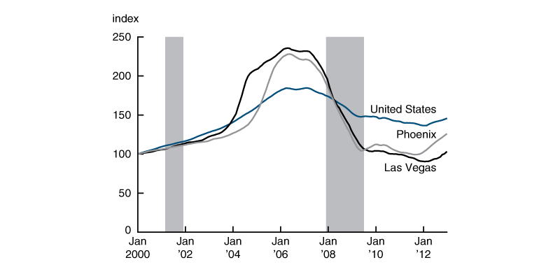
Source: S&P Global, S&P Dow Jones Indices, from the Federal Reserve Bank of St. Louis, FRED (Federal Reserve Economic Data).
The key aspects of the two booms I just highlighted are also apparent in other asset booms. For example, in the late 1980s, Norway, Sweden, and Finland all experienced stock market and real estate booms; indexes that combine equity and housing prices compiled by Borio, Kennedy, and Prowse (1994) more than doubled in these countries over a period of five years before all of the gains were erased. The eventual decline in asset prices in these countries was accompanied by a severe economic contraction and a banking crisis, which were especially acute in Finland. Similarly, Japan experienced stock market and real estate booms starting in the mid-1980s, but gave up most of the gains in stock and housing prices in the subsequent busts. These busts were also followed by a period of slow output growth in Japan known as the “Lost Decade.” Given the absence of widely agreed-upon business cycle dates outside the United States, I do not provide analogous figures on asset prices and recession dates for these episodes, although the episodes appear to follow a similar path.
Going back further in time, the United States experienced a major stock market boom in the 1920s—in the years leading up to the Great Depression. Figure 3 depicts the U.S. Dow Jones Industrial Average for the period surrounding the Great Depression.7 Starting in 1925, the Dow Jones index more than tripled over a period of four years. These gains were then wiped out in the span of two years following the infamous stock market crash in October 1929. As evident in the figure, the NBER dates the beginning of the Great Depression to August 1929, just before the stock market crash.
Figure 3. Dow Jones Industrial Average, January 1922–December 1936
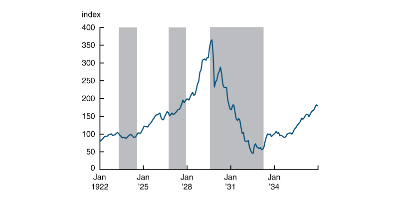
Source: S&P Global, S&P Dow Jones Indices, from the Federal Reserve Bank of St. Louis, FRED (Federal Reserve Economic Data).
Looking even further back, there are several well-known asset booms from the seventeenth and eighteenth centuries. These are reviewed in Garber (2000). Perhaps the most infamous of these is the Dutch Tulip Mania of 1636–37, in which prices of tulip bulbs supposedly rose to spectacular heights and then crashed. However, Garber argues that there is limited evidence on tulip bulb prices from this period and that some of the claims about this episode conflate the prices of especially rare bulbs, which remained high throughout the period, with those of cheaper regular varieties, whose prices increased but to much lower levels. Two better-documented episodes involve the prices of equity shares in private corporations—the French Mississippi Company (which was renamed the Company of the West and then the Company of the Indies) and the British South Sea Company. Prices of shares in both companies shot up by a factor of nearly ten over the course of a year and then crashed in 1720. While these episodes involve the familiar boom-and-bust pattern in asset prices from more-recent periods, the absence of national income accounts data from this time makes it hard to gauge if these episodes were similarly associated with large-scale contractions in economic activity. For the case of the Mississippi Company, Velde (2009) compiles data on the number of working looms and bolts of cloth produced in France, which can be used as a proxy for economic activity. While Velde focuses on changes in monetary policy that occurred several years later, his data extend to before and during the boom in the price of shares in the Mississippi Company, and they suggest there was indeed a significant but short-lived contraction in the second half of 1720.
From booms to bubbles
So far, I have been careful to describe episodes such as those illustrated in figures 1–3 as asset booms rather than bubbles, although these episodes have often been dubbed “bubbles” by the popular press and even by many economists. This is because I want to use the term bubble in the narrow sense that economic theorists use it; I will go on to argue that it may be reasonable to model these historical episodes as bubbles in line with this narrow definition.
One reading of episodes such as those depicted in figures 1–3 is that asset prices in these cases surged to levels that were far too high and that could not be sustained for very long. This interpretation is advanced by both Kindleberger (1978), in his influential book on financial crises, and Minsky (1986), in his work on the financial instability hypothesis. This argument relies on how most, if not all, of the price gains during the boom phase in these episodes were subsequently wiped out. Asset prices then remained at a lower level for a considerable period after the crash. Prices of assets during the booms seem aberrant and not in line with how traders valued these assets either before or after these booms.
To be sure, this is not the only way to interpret these episodes. In principle, there may have been one event that caused asset prices to rise and another event that caused them to later fall. Garber (2000) argues that there may have been valid reasons for people to expect the Mississippi Company and the South Sea Company to have been profitable; this can explain part of the rise in their stock values. More recently, Chodorow-Reich, Guren, and McQuade (2021) argue that the strong recovery in U.S. house prices since the mid-2000s suggests house price growth from 2000 onward was driven by fundamental forces, such as improvements in city-level amenities, shifts in demographics, and predicted wage growth. That is, certain cities became particularly attractive places to live in during this period, as evidenced by their higher house prices by 2020, and house prices grew more in those cities relative to house prices in other areas. At the same time, Chodorow-Reich, Guren, and McQuade also argue that explaining the rapid rise in house prices in those cities back in the early 2000s necessitates that homebuyers were overly optimistic at the time relative to what the fundamentals suggested. Indeed, in many historical asset booms, it is difficult to identify a change in some fundamental factor that can fully justify the high valuations at which assets were trading. Thinking about these episodes as situations in which an asset price is at too high of a level seems like, at the very least, a possibility whose policy implications are worth exploring.
Modeling asset booms as situations in which prices rise too high requires a coherent notion of what it means for an asset price to be too high. Determining after the fact that the asset must have been overvalued because its price eventually collapsed is not useful if policymakers must decide during the run-up whether to intervene. Moreover, using the subsequent outcome does not offer a precise explanation of what “too high” means or at what point prices become too high. What’s needed is a benchmark value for an asset that can tell us when the price should be deemed to be too high. Economic theorists have proposed the present discounted value of the cash flows or dividends that an asset is expected to yield over its lifetime as one such benchmark. Let $d{_t{_+}_s}$ denote the dividend paid by an asset at date t + s. Suppose that in addition to the asset, agents can invest in fixed-income securities that pay an interest rate of $R{_t{_,}{_t}{_+}_s}$ at date t + s for each dollar invested at date t. This ability to invest in these fixed-income securities provides a way to translate dollars in the future into dollars today, given that having a dollar at date t + s requires setting aside \(\frac{1}{1\,+\,{{R}_{t,t+s}}}\) dollars at date t. I define the fundamental value of the asset ${f_t}$ at date t as the expected discounted dividends valued in present dollars:
$1)\quad{{f}_{t}}={{E}_{t}}\left[ \sum{_{s=0}^{\infty }}\frac{{{d}_{t+s}}}{1+{{R}_{t,t+s}}} \right].$
Armed with this benchmark, I can define a bubble as a situation in which the price of the asset $p{_t}$ at some date t is different from its benchmark of fundamental value $f{_t}$ as defined in equation 1. When using this notion to think about asset booms, the relevant scenario is where the price $p{_t}$ strictly exceeds $f{_t}$. Such a scenario offers a concrete sense in which the price of an asset can be too high. However, just because the asset’s price exceeds its fundamental value does not necessarily imply such a price is unsustainable and must eventually collapse. Indeed, it is not obvious such a prediction would be desirable when, historically, not all asset booms have ended in busts.8 In the models I discuss in the next section, asset prices collapse in some states of the world but not in others. It seems reasonable to define a bubble as a situation in which an asset is overvalued without presupposing its prices must crash. That said, in the models I describe in the following section, bubbles are vulnerable to collapse, and nothing ensures a bubble must last indefinitely.
If historical asset booms correspond to bubbles as I have defined them, one should be able to infer the appropriate policy response to such booms by writing down a model that gives rise to a bubble and then studying its policy implications. But this proposition turns out to be difficult. In the simplest models that one can write down, assets cannot trade at a price that differs from their fundamental value. Intuitively, a trader who intends to hold on to an asset for as long as it pays out dividends will not pay more for an asset than the present discounted value of the dividends it is expected to pay. The trader might be willing to pay more than they expect it to generate in dividends if they intend to sell the asset later at a high price. But this begs the question of why the agent should reasonably expect someone else to overpay for the asset. When all agents are rational and assume others are rational, as economic models commonly assume, it will be hard to get an equilibrium bubble. Before thinking about what policy should do in the face of a bubble, one must first figure out when bubbles are even possible.
Modeling bubbles
In Barlevy (2018), I reviewed a variety of situations in which economists have shown that bubbles can arise. The theme of that article was that research on bubbles had primarily focused on establishing that bubbles were possible and, as a result, had yet to satisfactorily address some of the key questions about bubbles that interested policymakers. That observation can explain why models of bubbles seem to have attracted only limited interest in policy circles. But I further argued that existing models had developed sufficiently when I wrote that article to begin exploring these questions, and encouraged economists to start to tackle them. As I discuss later, more-recent research has started to rise to this challenge. But I first review the models that economists have shown can generate bubbles to set up my discussion of the more-recent work.
In the late 1950s, Samuelson (1958) first demonstrated that an asset could trade above its intrinsic value in his overlapping-generations model of money.9 In that model, an intrinsically worthless asset like paper money could trade at a positive price if agents wish to save but have no assets other than paper money to do so. The value of money (in terms of goods) is thus positive, even though money pays no dividends. This model was long regarded as a theory of money rather than a framework for studying asset booms. Diamond (1965) built on Samuelson’s model by introducing capital as a durable factor of production that agents could use to save. He interpreted the possibility of an intrinsically worthless asset trading at a positive price not as money but as government debt that is perpetually rolled over and financed with new debt issuance rather than with taxes. Tirole (1985) later pointed out that the same framework could be used to study asset booms. As Diamond (1965) and Tirole (1985) explain, the reason an intrinsically worthless asset that pays no dividends can trade at a positive price even when agents can hold other assets, such as physical capital, is that the equilibrium in which the price of such an asset is zero is dynamically inefficient. That is, absent the bubble asset, the economy would grow faster than the equilibrium interest rate on the asset that agents can hold. In that case, agents would prefer to buy an intrinsically worthless asset that pays no dividends if its price grew at the same rate as the economy, as it indeed could if agents spend a nonvanishing share of their growing income on the asset. A large literature has subsequently explored the bubbles that arise in these models and whether they can resemble asset booms and busts from the historical episodes described earlier in this article. Models of bubbles based on dynamic inefficiency have declined in popularity over time, in part because of evidence by Abel et al. (1989) that questioned whether dynamic inefficiency was empirically plausible; however, such models continue to be used in some applications, including most recently in Galí (2014, 2021).10
A drawback of models of bubbles based on dynamic inefficiency is that they imply bubbles crowd out capital. A corollary of this result is that when bubbles collapse, capital accumulation and output should both rise. By contrast, historical asset booms are associated with higher investment—be it the creation of new technology firms or the construction of new housing—and the end of these booms is associated not with higher output, but with depressed output. This historical pattern led to the development of a different class of models of bubbles that relies on credit market frictions rather than dynamic inefficiency.11 In these models, entrepreneurs who produce capital goods are limited in how much they can borrow to secure the inputs they need for production. Intrinsically worthless assets that pay no dividends may trade at positive prices in these models—either 1) when entrepreneurs can borrow against these assets and so have an incentive to accumulate them or 2) if less productive entrepreneurs can buy these assets and then sell them later on when these same entrepreneurs become more productive and would like to borrow to produce more. Bubbles in this case can encourage capital accumulation. This approach has been developed by Caballero and Krishnamurthy (2006), Martin and Ventura (2012), Farhi and Tirole (2012), Hirano and Yanagawa (2017), and Miao and Wang (2018), among others. These papers in turn build on earlier work by Kocherlakota (1992) and Santos and Woodford (1997) on bubbles associated with borrowing constraints for households.
Despite their different implications for investment, models of bubbles based on dynamic inefficiency and those based on credit market frictions have several aspects in common. Both involve bubbles that must potentially last indefinitely; if there were a finite date beyond which the value of the bubble must be zero, agents would refuse to pay a high price for the asset one period beforehand, and the original price path would unravel. Additionally, in both models, bubbles act to correct the underlying distortion that allows a bubble to arise in the first place: Bubbles let agents earn higher returns when the economy is dynamically efficient absent the bubble, and they allow financially constrained capital producers to secure the inputs they need but cannot borrow when there are financial frictions. A distinct line of research has explored the possibility of bubbles that need not survive indefinitely nor correct the underlying inefficiency that allows them to occur in the first place. This literature focuses on the role of private information about the asset.12 The first model along these lines was developed by Allen, Morris, and Postlewaite (1993), with follow-up work by Conlon (2004), Doblas-Madrid (2012), and Awaya, Iwasaki, and Watanabe (forthcoming), among others.
In models based on private information, individuals might be willing to pay more for an asset than they know it is worth because they hope to sell it at an even higher price to someone who is unaware the asset is overvalued. For this reason, these models are sometimes called greater-fool models.13 Formally, these models feature a state of the world in which all agents know the asset is overvalued and so the asset can be viewed as a bubble. But there are also other states of the world in which not all agents know the asset is overvalued. In the state where the asset is a bubble, some agent will eventually refuse to buy the asset, and at that point the asset price will fall. Hence, unlike in models of bubbles based on dynamic inefficiency or credit constraints, in these models a bubble must collapse in finite time. Moreover, in the state of the world where the asset is overvalued, there is no benefit to letting agents trade the asset between them as there is in models with dynamic inefficiency or credit market frictions. Agents trade the asset because they are unsure what others know, not because of mutual gains from trade.
Another example of a model of bubbles that need not last indefinitely nor correct the friction that allows them to occur in the first place assumes that traders borrow to buy assets and that their lenders cannot easily monitor what borrowers are doing. In this case, traders might be willing to buy a risky asset at a price that exceeds the expected payoff from these assets, knowing they can pass any losses on to their lenders if the realized return on the asset is low. The asset would trade at a price that reflects the highest returns the asset could pay out rather than the returns the asset is expected to pay out. Accordingly, these models are known as risk-shifting models of bubbles. Lenders would naturally want to avoid lending to agents who speculate at their expense, so it is essential that they cannot identify what borrowers are doing. Risk-shifting models thus require private information just as greater-fool models do, although the information is not about what the asset is worth or what other traders know, but about what assets borrowers are investing in. These models were first developed by Allen and Gorton (1993) and Allen and Gale (2000), with follow-up work by Barlevy (2014), Dow and Han (2015), and Bengui and Phan (2018).
Finally, there is a behavioral finance literature that considers economies in which agents bid up asset prices because they hold overly optimistic beliefs about assets. An important paper in this literature is Scheinkman and Xiong (2003), who posit that traders place too much confidence in the precision of their own information relative to the information that others receive. When there are restrictions on selling assets short, it will be the most optimistic agents who determine asset prices. This is because when short-selling is prohibited, pessimistic agents will sell their assets and leave the market, even though they may have wanted to bet against an asset they view as overvalued. The price of the asset will then reflect the views of the remaining agents, who are more optimistic than the ones who left. If the agents who stayed in the market are overconfident, their view of the asset is likely to be inflated, and the asset price will tend to exceed its true underlying fundamental value. Moreover, since traders understand that they will be able to sell assets in the future at a high price to others if they happen to receive more favorable information, traders will be willing to pay more for the asset than they believe it is worth.14 Subsequent work has explored other psychological biases that can lead agents to be overly optimistic about assets. Recent examples include Barberis et al. (2018) and Bordalo et al. (2021), who consider the tendency of agents to extrapolate either from recent price dynamics or from salient price changes to form expectations of future prices.
In short, there are various scenarios that allow bubbles to occur. Some of the papers I cited do explore a role for policy in these models. However, as I argued in Barlevy (2018), the existing literature, at least as of 2018, had yet to adequately address the key questions that policymakers were specifically interested in. To briefly summarize, policymakers familiar with episodes like those illustrated in figures 1–3 worry that an unchecked asset boom may give way to a collapse in asset prices and a potentially nasty recession. What they want to know is whether to intervene when they see an asset boom—and if so, how. If an eventual collapse in asset prices triggers a recession, would an early intervention also trigger a recession, or would it soften the blow that would occur following an even bigger collapse in asset prices? If early intervention against asset booms is in fact warranted, what is the best intervention? Should it involve raising interest rates, imposing regulatory restrictions, or both? To put it another way, what policymakers want to know is whether they should lean, screen, or clean—that is, lean against the boom by raising interest rates; engage in stricter screening and oversight of financial intermediaries that lend against these assets to limit how much they can lend or at what terms; or wait to see what happens and, if necessary, clean up by stimulating economic activity after a collapse in asset prices. While the available literature at the time I wrote my 2018 article had yet to provide satisfactory answers to these questions, I made the case that models of bubbles had developed sufficiently that they could begin to tackle them, and encouraged researchers working in this area to proceed in that direction.
Exploring policy in risk-shifting models of bubbles
Besides encouraging others to explore the questions that policymakers concerned about asset booms are most interested in, I proceeded to explore these questions in some of my own research. The result of these efforts is described in Allen, Barlevy, and Gale (2022), which explores the effects of intervention in risk-shifting models of bubbles. Risk-shifting models seem particularly well suited for studying these questions, since credit in these models is essential for a bubble to occur, meaning that credit restrictions have the potential to eliminate bubbles.
To be clear, risk-shifting models are not unique in allowing a role for credit. Researchers have introduced credit into other models of bubbles as well. For example, Doblas-Madrid and Lansing (2016) allow for credit in a greater-fool model of bubbles and show that it governs the pace of asset price growth during the boom. Geanakoplos (2010) and Simsek (2013) consider the effects of leverage in models where not all agents are equally optimistic about the asset, and show that credit can amplify the extent of overvaluation by allowing more funds to flow into the hands of those who hold the most optimistic views about the asset. There is also work that adds limited amounts of credit to models of bubbles based on credit market frictions. See Martin and Ventura (2016) as an example of such analysis.15 In such a case with limited amounts of credit added, bubble assets serve as a substitute to lending for agents with more resources than they need but a limited ability to lend, so easing credit constraints may actually lower demand for bubble assets. What makes risk-shifting models distinct is that credit doesn’t just affect the demand for bubble assets but is the reason bubbles arise in the first place.
Let me sketch the key features of the Allen, Barlevy, and Gale (2022) model. As in other risk-shifting models, borrowers can undertake two activities—one that is safe and one that is risky; my co-authors and I model these activities as borrowing to buy inputs for production using a riskless technology and borrowing to buy an existing risky asset from someone initially endowed with the asset, respectively. Borrowers differ in their productivity in operating the technology, and only they know their own productivity. The most productive entrepreneurs can earn higher returns from operating the riskless technology than lenders can earn on their own, so there is scope for gains from trade between lenders and the most productive entrepreneurs. Less productive entrepreneurs cannot profit from borrowing to produce, but they might still profit from borrowing to buy risky assets: If the realized return on the risky asset is high they can keep some profits, and if it is low they can default and shift their losses to the creditors. Lenders cannot observe the productivity of any given borrower and so cannot restrict their lending to the most productive borrowers. This setup can be viewed as a metaphor for any scenario in which borrowers engage in activities associated with different levels of risk that are hard for outsiders to distinguish. For example, some people might borrow to buy a home they intend to live in regardless of what happens to housing prices (and so are safe to lend to), while others borrow to speculate on house prices, selling the house if its price rises and defaulting if it falls (and so are riskier to lend to).
As in previous risk-shifting models of bubbles, private information about what borrowers do with the funds they secure allows the risky asset to trade above its expected value. Less productive entrepreneurs will borrow to buy the risky asset (rather than to produce) and bid up the asset price. We consider a regime-switching process for the asset’s dividends, in which dividends start out high in the initial regime and then fall permanently when the regime switches. During the initial regime, less productive entrepreneurs will borrow to buy the asset and gamble that dividends next period will be high. When the regime changes and dividends are low, agents who borrowed to buy the risky asset default and the asset price will fall. Since there is no remaining uncertainty to gamble on at this point, speculation ends. Under some additional assumptions about how dividends behave in the initial regime, the bubble (and the price of the asset) will grow during the initial regime while the asset is overvalued.16
In Allen, Barlevy, and Gale (2022), we assume default is costly—this is a key feature that distinguishes our risk-shifting model from previous ones. For simplicity’s sake, we model the costs from default as collection costs: Lenders must expend resources to collect from defaulting borrowers. While collection costs may be modest in practice, default is likely associated with various additional indirect costs. For example, default may lead to debt overhang for lenders that prevents them from issuing new loans in the future, resulting in forgone profits for lenders above and beyond the direct collection costs.17 In addition, financially distressed borrowers may engage in various activities that harm others. For instance, they may liquidate their assets to pay lenders, and these fire sales can reduce the value of similar assets held by other agents. Alternatively, borrowers may default on their suppliers as well as their lenders. In all of these cases, borrowers do not bear the full consequences of their speculative activity. We model default costs as pure waste; thus, a regime switch can be viewed as triggering not only a drop in asset prices and defaults by agents who borrowed against the asset, but also a recession in which agents have fewer resources left to consume after accounting for default costs.
The default costs we posit are proportional to the amount that was lent out, since lenders must incur larger costs when there is more money to go after. The indirect costs of default we discuss would similarly be larger the more agents borrow because the collateral damage of financial distress will be larger the more agents originally borrowed to speculate. This implies that the recession triggered by the regime switch that leads speculators to default will be more severe, the larger the amount of speculation and the higher the price of the asset during the initial boom. In that sense, a larger asset boom may sow the seeds for a more severe recession later on.
Given that borrowers do not bear all of the default costs they create in Allen, Barlevy, and Gale (2022), the laissez-faire equilibrium in our model will be inefficient. Intuitively, speculation serves no socially useful purpose: A speculator who buys an asset from the agent originally endowed with it earns the same return as the original owner. While borrowing to buy a risky asset from its original owner creates no surplus, it does impose a deadweight loss on society: If agents borrow to buy the asset and then default, society is poorer. We confirm that the equilibrium is inefficient by considering the effects of a quota on total lending in our model.18 Under such a quota, the most productive entrepreneurs would bid up the interest rate to secure all available funding. Lenders would then have to use any remaining wealth to buy the risky asset directly, since they can offer no more loans. This will push up the price of the risky asset and drive down its return, rendering speculation unprofitable for remaining entrepreneurs. A quota induces lenders to buy assets directly rather than lend to others to do so.
We can set the quota to ensure that all of the entrepreneurs who originally chose to produce in the laissez-faire equilibrium still borrow to produce under the quota. Such a quota ensures that would-be lenders spend the same amount of their own wealth on the asset that speculators would have borrowed to spend on the asset in the laissez-faire equilibrium. The quota can thus eliminate speculation without changing asset prices or interest rates. The most productive entrepreneurs will be just as well off as under the original equilibrium because they face the same interest rate. Less productive entrepreneurs are no worse off because in the original equilibrium they earned zero profits from speculation (or else demand for borrowing would have been infinite). The original asset owners are just as well off, given they receive the same price for the asset. But lenders will be strictly better off by avoiding default costs. Effectively, lenders are spared from a recession that could have happened if agents were allowed to speculate during the boom.
Even if policymakers cannot eliminate speculation altogether in our model, it might be possible to mitigate the recession that would happen when the asset price crashes by reducing the asset price during the boom. This is possible because default costs are proportional to the amount agents borrow to buy the risky asset, so reducing the asset price reduces the amount that less productive agents borrow to buy the asset. One way to drive down asset prices is with contractionary monetary policy. Such a policy makes lenders temporarily poorer and less willing to lend. The implied default costs will then be smaller. While mitigating the recession this way requires making agents poorer today, such a trade-off may be desirable if it avoids large default costs.
Policymakers in our model thus have a reason to intervene during an asset boom. However, the case for intervention I just described does not hinge on the boom being associated with an asset bubble. The benefit of intervention comes from avoiding costly speculation, not from mitigating overvaluation. Given a price for the asset, whether the fundamental value of the asset is equal to this price or lies below it is irrelevant for why avoiding speculation is beneficial. Likewise, the argument for intervening to lower the price of the asset does not depend on whether such an intervention would also reduce the fundamental value. To be sure, if we hold the fundamental value of an asset fixed in our model, a larger bubble would imply more borrowing and larger default costs. Other things being equal, then, bubbles can make a boom more costly. But that doesn’t mean the asset must be a bubble for intervention to be desirable. In Allen, Barlevy, and Gale (2022), we confirm this formally by showing that in certain situations, less productive agents might engage in speculation even when the asset price is not overvalued, and the case for intervention applies equally under those circumstances.
Alternative models of bubbles
A key lesson from Allen, Barlevy, and Gale (2022) is that determining whether an asset is a bubble is not essential for making the case for acting against a boom to avoid a costly recession when the asset boom ends. It is natural to ask whether this result is only true for risk-shifting models of bubbles. Research on other models of bubbles has not explicitly discussed this matter, but my reading of the literature suggests that intervening to avoid a recession can be desirable in these models as well, even when assets are not bubbles.
Consider models of bubbles based on excessive optimism. Economists have recently started to look at whether there might be scope for interventions against asset booms of this type, at least under certain circumstances. As I noted earlier, several authors have studied the effects of allowing for credit in these models. Caballero and Simsek (2020) explore whether lending by pessimists to optimists can create potential problems that merit policy action when agents hold different views about assets. Farhi and Werning (2020) explore the effects of policy when the agents who borrow to buy assets extrapolate from recent asset returns in forming their expectations of future returns, just as in Bordalo et al. (2021). Rather than letting agents disagree about the asset, Farhi and Werning assume that some agents have access to asset markets and others do not. This creates scope for agents shut out of the asset markets to lend to those who do have access, as those shut out of asset markets seek higher returns.
Importantly, both Caballero and Simsek (2020) and Farhi and Werning (2020) also assume that goods prices are rigid. This means that a negative economic shock, such as one that implies lower returns on the asset, can lead to a recession given that goods prices cannot fully respond to the shock. In this situation, intervention during the boom can have ramifications for the price of the asset during the recession, which in turn has implications for how severe the recession might be.
The results in Caballero and Simsek (2020) and Farhi and Werning (2020) mirror those that I found in my own work on risk-shifting. In the risk-shifting model of Allen, Barlevy, and Gale (2022), lending during the asset boom leads to a more severe recession once the boom ends because default costs are proportional to the amount agents borrow to speculate. In models with rigid goods prices and either disagreement or extrapolative beliefs, lending during the boom also leads to more severe recessions if a negative economic shock occurs. The reason is as follows. In Caballero and Simsek (2020), optimists who borrow to buy the asset must sell their asset holdings to repay their loans when a negative shock occurs. Since optimists no longer hold the asset after the negative shock, the asset price will fall. A lower price of the asset will lead to lower demand for goods during the recession as the agents who hold the asset now feel less wealthy. This fall in aggregate demand results in a more severe recession. A similar result occurs in the model of Farhi and Werning (2020). More lending during the boom pushes the asset price up. This means that if a negative shock occurs and triggers a recession, agents who extrapolate from past returns will see a larger fall in the price of the asset during the recession and turn more pessimistic about future returns. Their reluctance to hold the asset will result in a lower asset price during the recession, just as in Caballero and Simsek’s model.
While neither Caballero and Simsek (2020) nor Farhi and Werning (2020) point this out, the aggregate demand externalities that I’ve described do not depend on whether the agents who hold the asset during the boom are overly optimistic about its returns. Even when these agents are correct in their assessment of the probability of a low return on the asset, reducing leverage during the boom will help increase asset prices during the recession. Should policymakers learn that the agents who buy the asset in the boom have a correct assessment of the returns on the asset so that the asset price reflects its true underlying fundamentals, they would still want to reduce lending during the boom in order to push up the price of the asset during the recession, increase agent wealth, and stimulate demand for goods.
Next, consider models of bubbles that arise because of credit market frictions. Recent work by Biswas, Hanson, and Phan (2020) has explored whether policymakers should intervene to mitigate a possible recession in those models. They introduce downward wage rigidity into an otherwise standard model of bubbles based on credit market frictions. While a bubble that can be sustained indefinitely improves welfare in their setting by allowing entrepreneurs to secure the resources they need, they show that a bubble that cannot be sustained indefinitely may be harmful. The logic is as follows. During the boom, the bubble allows entrepreneurs to produce more capital. A higher capital stock increases the marginal product of labor, and so wages rise during the boom. When the bubble bursts, entrepreneurs can no longer create as much capital, and the marginal product of labor falls. Downward wage rigidity prevents the wage from falling immediately. Firms will then reduce their hiring, resulting in a recession once the bubble bursts. If the recession is sufficiently severe or lasts sufficiently long, the cost of forgone output after the bubble collapses may more than offset the benefits of higher capital during the boom.
The argument for dampening the initial boom in their model is similar in spirit to the one for models of bubbles based on risk-shifting or excessive optimism with leverage. While a boom in Biswas, Hanson, and Phan (2020) can only occur when there is a bubble, the logic of their argument extends to any scenario that leads to a temporary increase in capital accumulation. Consider, for example, a temporary productivity shock that creates an incentive for agents to accumulate capital. If agents accumulate capital, that would drive up the marginal product of labor and hence the wage. But when the shock dissipates and capital depreciates, wage rigidity will imply the wage is too high. The economy will then undergo a recession until wages fall sufficiently. Just as there is a reason to curb lending for the sake of mitigating the subsequent recession in the two other types of models of bubbles, here there would be an incentive to limit capital accumulation in response to the productivity shock.19
There is a common thread through all of these examples. The case for policy intervention hinges on the idea that letting an asset boom go unchecked leads to bad subsequent outcomes. This can be because the boom is associated with lending that creates negative externalities if and when asset prices collapse or because the boom leads to higher wages, which later serve as a drag on economic activity. None of these arguments hinge on asset prices exceeding fundamentals. The purpose of intervention is to correct the distorting effects of the boom, and these distortions occur whether the boom is associated with a bubble or not. The intervention itself may potentially be costly: If policymakers cannot eliminate speculation, they may have to resort to contractionary monetary policy that reduces current output. Curbing lending between optimists and pessimists may prevent the agents who value the asset the most from owning all of it. Preventing productive agents from producing capital will reduce output. However, these costs may be justified if leaving an asset boom alone would result in a painful recession later on.
Policymakers might therefore not need to determine if the booms they face are associated with bubbles to justify acting during an asset boom. However, this does not mean that policymakers should automatically intervene whenever there is a boom. If there is no large-scale borrowing against the asset whose price is increasing or if the boom is not associated with high wages that are expected to remain high when the boom ends, there may not be a reason to intervene. Even if the boom may sow the seeds for a subsequent recession, intervention may still not be desirable. Here, the work by Biswas, Hanson, and Phan (2020) is particularly instructive: In their model, intervention would only be justified if the asset boom is likely to collapse. Determining how likely an asset is to collapse may be conceptually just as hard as determining its fundamental value. So gauging the appropriate response to an asset boom may be challenging. Nevertheless, the analysis in Biswas, Hanson, and Phan (2020) suggests the type of data policymakers should be looking at—that is, data on what agents expect asset prices to be in the future.
Conclusion
Models of asset bubbles—that is, models in which the price of an asset is detached from the underlying fundamentals—seem natural and appropriate for studying asset booms. With that said, whether an asset is a bubble may not matter in determining whether policymakers should intervene during a boom to mitigate the fallout should the boom turn into a bust. Given that I myself have advocated for using models of bubbles to study appropriate policy during asset booms of the past, I feel repentant in contributing to the perception that appropriately responding to booms requires knowing whether a boom corresponds to a bubble.
At the same time, I am not advocating for abandoning models in which the price of an asset is detached from fundamentals. The notion that assets can trade at a price that does not reflect their fundamentals remains important for a host of reasons, including for policy questions that do not involve acting against bubbles to mitigate a potential recession when they collapse.
One theme that emerges from work on asset bubbles is that they only arise when the initial allocation in the economy is inefficient and agents stand to gain from trading with one another. Indeed, all of the models of bubbles I discussed feature some type of inefficiency. Knowing that there are bubbles in asset markets could therefore alert policymakers to the presence of some underlying inefficiency, even if this information is not important for whether they should intervene against an asset boom to avoid an eventual recession. Overvaluation can also lead to a misallocation of resources and to the creation of assets that may not benefit society. Even if policymakers do not need to know whether an asset is overvalued to mitigate the consequences of a collapse in asset prices, they might still need to know if the asset is overvalued to gauge whether they should discourage the creation of assets that are less valuable to society than their price suggests. Whether they should discourage asset creation or not will depend on the reason bubbles arise. Recall that bubbles tend to correct the underlying friction that gives rise to them in models based on dynamic inefficiency and credit market frictions, but not in greater-fool or risk-shifting models. Figuring out all of the different implications of these models remains an important direction for future research.
Finally, while many unanswered questions about bubbles remain, the irrelevance of the notion of bubbles for certain policy questions suggests economists might want to study models of asset booms that do not involve bubbles. Asset booms in which the underlying assets are arguably not bubbles can still be useful for policy analysis, and may help to get at issues that existing models of bubbles ignore.20 Models of bubbles have their place, but they should not be viewed as the only way to represent or understand asset booms.
Notes
1 Details on the NBER’s Business Cycle Dating Committee are available online.
2 Ventura said this in a panel session at a conference on bubbles in Barcelona sponsored by the CREI (Centre de Recerca en Economia Internacional) in October 2017; Ventura’s remark at this conference is recorded in Barlevy (2018).
3 Early discussions about the possibility of a financial stability mandate include Bean et al. (2010), Mishkin (2011), and the Bank for International Settlements, Study Group (2011).
4 For a discussion of how financial stability concerns matter for output and inflation, see Ajello et al. (2022).
5 The Nasdaq-100 comprises the 100-plus largest nonfinancial firms listed on the Nasdaq Stock Market, according to market capitalization; further details on the Nasdaq-100 are available online.
6 Officially, these indexes are called the Standard and Poor’s (S&P) CoreLogic Case-Shiller Home Price Indices; further details on them are available online.
7 Details on the Dow Jones Industrial Average are available online.
8 For example, Greenwood, Shleifer, and You (2019) show that among industries that experienced a 100 percent price run-up over a two-year period, only slightly more than half saw a price crash—that is, a price drop of at least 40 percent over the next two years.
9 Allais (1947) independently developed the overlapping-generations model a decade earlier, but his analysis was not as widely known nor as influential.
10 Geerolf (2018) revisits the Abel et al. (1989) evidence and argues that dynamic inefficiency may be plausible for some countries after all.
11 Olivier (2000) shows that growth-enhancing bubbles can occur in a model with only dynamic inefficiency if we replace capital with research and development (R&D) that uses labor. If bubbles are associated with the claims on profits from patents, the presence of bubbles would encourage people to shift from production to R&D.
12 Strictly speaking, these models require not just private information, but also a reason unrelated to information for agents to trade. Intuitively, unless there is a reason beyond information for agents to trade, agents would be reluctant to trade knowing others have private information that makes them willing to take the opposite side of the trade. Tirole (1982) showed that private information on its own cannot give rise to a bubble—that is, a bubble cannot occur when agents have no other reason to trade and agree on the underlying model before learning their private information.
13 For a more extensive review of the literature on greater-fool bubbles, see Barlevy (2015).
14 Harrison and Kreps (1978) were the first to demonstrate that traders will value an asset more than they believe its dividends are worth when they expect others will eventually turn more optimistic than them; but notably, their model did not assume any overconfidence.
15 Martin and Ventura (2016) assume state-contingent debt to avoid dealing with default, so in their framework there is no problem when agents who borrowed to buy assets suffer losses. This contrasts with the work on risk-shifting models, in which the possibility of agent default plays a crucial role.
16 Specifically, for the bubble to grow before it crashes, dividends must start low and rise only if the economy remains in the initial regime for a sufficiently long period. For example, a firm might earn temporarily high profits if a new patent is workable, which takes time to establish. In this case, early in the initial regime, agents speculate not on whether the dividends next period will be high, but on whether the patent will remain viable next period and the asset price will rise.
17 The costs would be borne not just by lenders but also by their potential future borrowers, who would be unable to secure funds. For more on the debt overhang channel, see Philippon (2010).
18 In principle, we could have considered a tax on lending that is a rebated lump-sum to lenders. That is, rather than forbidding agents from lending above a certain amount in total, we can tax their lending until lending becomes sufficiently unattractive such that agents voluntarily choose to buy the risky asset.
19 I am indebted to Tomohiro Hirano for alerting me to this point.
20 For example, in Barlevy (2015) I argued that models such as Harrison and Kreps (1978) that assume agents hold different beliefs but are not overly optimistic should not be interpreted as models of bubbles. That does not mean these models aren’t useful for studying asset booms. Indeed, these models are useful for understanding trade volumes, and I myself have used them to study asset booms in Barlevy (2021).
References
Abel, Andrew B., N. Gregory Mankiw, Lawrence H. Summers, and Richard J. Zeckhauser, 1989, “Assessing dynamic efficiency: Theory and evidence,” Review of Economic Studies, Vol. 56, No. 1, January, pp. 1–19. Crossref
Ajello, Andrea, Nina Boyarchenko, François Gourio, and Andrea Tambalotti, 2022, “Financial stability considerations for monetary policy: Theoretical mechanisms,” Federal Reserve Bank of Chicago, working paper, No. 2022-06, February. Crossref
Allais, Maurice, 1947, Économie et intérêt: Présentation nouvelle des problèmes fondamentaux relatifs au rôle économique du taux de l’intérêt et de leurs solutions, 2 vols., Paris: Imprimerie nationale.
Allen, Franklin, Gadi Barlevy, and Douglas Gale, 2022, “Asset price booms and macroeconomic policy: A risk-shifting approach,” American Economic Journal: Macroeconomics, Vol. 14, No. 2, April, pp. 243–280. Crossref
Allen, Franklin, and Douglas Gale, 2000, “Bubbles and crises,” Economic Journal, Vol. 110, No. 460, January, pp. 236–255. Crossref
Allen, Franklin, and Gary Gorton, 1993, “Churning bubbles,” Review of Economic Studies, Vol. 60, No. 4, October, pp. 813–836. Crossref
Allen, Franklin, Stephen Morris, and Andrew Postlewaite, 1993, “Finite bubbles with short sale constraints and asymmetric information,” Journal of Economic Theory, Vol. 61, No. 2, December, pp. 206–229. Crossref
Awaya, Yu, Kohei Iwasaki, and Makoto Watanabe, forthcoming, “Rational bubbles and middlemen,” Theoretical Economics, available online.
Bank for International Settlements, Study Group, 2011, Central Bank Governance and Financial Stability, report, Basel, Switzerland, May, available online.
Barberis, Nicholas, Robin Greenwood, Lawrence Jin, and Andrei Shleifer, 2018, “Extrapolation and bubbles,” Journal of Financial Economics, Vol. 129, No. 2, August, pp. 203–227. Crossref
Barlevy, Gadi, 2021, “On speculative frenzies and stabilization policy,” Federal Reserve Bank of Chicago, mimeo.
Barlevy, Gadi, 2018, “Bridging between policymakers’ and economists’ views on bubbles,” Economic Perspectives, Federal Reserve Bank of Chicago, Vol. 42, No. 4. Crossref
Barlevy, Gadi, 2015, “Bubbles and fools,” Economic Perspectives, Federal Reserve Bank of Chicago, Vol. 39, Second Quarter, pp. 54–76, available online.
Barlevy, Gadi, 2014, “A leverage-based model of speculative bubbles,” Journal of Economic Theory, Vol. 153, September, pp. 459–505. Crossref
Bean, Charles, Matthias Paustian, Adrian Penalver, and Tim Taylor, 2010, “Monetary policy after the fall,” in Macroeconomic Challenges: The Decade Ahead, proceedings of the Jackson Hole Economic Policy Symposium, Federal Reserve Bank of Kansas City, pp. 267–328, available online.
Bengui, Julien, and Toan Phan, 2018, “Asset pledgeability and endogenously leveraged bubbles,” Journal of Economic Theory, Vol. 177, September, pp. 280–314. Crossref
Biswas, Siddhartha, Andrew Hanson, and Toan Phan, 2020, “Bubbly recessions,” American Economic Journal: Macroeconomics, Vol. 12, No. 4, October, pp. 33–70. Crossref
Boissay, Frédéric, Fabrice Collard, Jordi Galí, and Cristina Manea, 2022, “Monetary policy and endogenous financial crises,” Centre de Recerca en Economia Internacional (CREI), working paper, January 7, available online.
Bordalo, Pedro, Nicola Gennaioli, Spencer Yongwook Kwon, and Andrei Shleifer, 2021, “Diagnostic bubbles,” Journal of Financial Economics, Vol. 141, No. 3, September, pp. 1060–1077. Crossref
Borio, Claudio, Neale Kennedy, and Stephen D. Prowse, 1994, “Exploring aggregate asset price fluctuations across countries: Measurement, determinants and monetary policy implications,” Bank for International Settlements, working paper, No. 40, April 2, available online.
Caballero, Ricardo J., and Arvind Krishnamurthy, 2006, “Bubbles and capital flow volatility: Causes and risk management,” Journal of Monetary Economics, Vol. 53, No. 1, January, pp. 35–53. Crossref
Caballero, Ricardo J., and Alp Simsek, 2020, “Prudential monetary policy,” National Bureau of Economic Research, working paper, No. 25977, revised March 2020 (originally issued June 2019). Crossref
Chodorow-Reich, Gabriel, Adam M. Guren, and Timothy J. McQuade, 2021, “The 2000s housing cycle with 2020 hindsight: A neo-Kindlebergerian view,” National Bureau of Economic Research, working paper, No. 29140, August. Crossref
Conlon, John R., 2004, “Simple finite horizon bubbles robust to higher order knowledge,” Econometrica, Vol. 72, No. 3, May, pp. 927–936. Crossref
Diamond, Peter A., 1965, “National debt in a neoclassical growth model,” American Economic Review, Vol. 55, No. 5, part 1, December, pp. 1126–1150, available online.
Doblas-Madrid, Antonio, 2012, “A robust model of bubbles with multidimensional uncertainty,” Econometrica, Vol. 80, No. 5, September, pp. 1845–1893. Crossref
Doblas-Madrid, Antonio, and Kevin J. Lansing, 2016, “Credit-fuelled bubbles,” Federal Reserve Bank of San Francisco, working paper, No. 2016-02, March. Crossref
Dow, James, and Jungsuk Han, 2015, “Contractual incompleteness, limited liability and asset price bubbles,” Journal of Financial Economics, Vol. 116, No. 2, May, pp. 383–409. Crossref
Farhi, Emmanuel, and Jean Tirole, 2012, “Bubbly liquidity,” Review of Economic Studies, Vol. 79, No. 2, April, pp. 678–706. Crossref
Farhi, Emmanuel, and Iván Werning, 2020, “Taming a Minsky cycle,” Massachusetts Institute of Technology, unpublished manuscript.
Galí, Jordi, 2021, “Monetary policy and bubbles in a New Keynesian model with overlapping generations,” American Economic Journal: Macroeconomics, Vol. 13, No. 2, April, pp. 121–167. Crossref
Galí, Jordi, 2014, “Monetary policy and rational asset price bubbles,” American Economic Review, Vol. 104, No. 3, March, pp. 721–752. Crossref
Garber, Peter M., 2000, Famous First Bubbles: The Fundamentals of Early Manias, Cambridge, MA: MIT Press. Crossref
Geanakoplos, John, 2010, “The leverage cycle,” in Macroeconomics Annual 2009, Daron Acemoglu, Kenneth Rogoff, and Michael Woodford (eds.), Vol. 24, Chicago: University of Chicago Press, pp. 1–66. Crossref
Geerolf, François, 2018, “Reassessing dynamic efficiency,” University of California, Los Angeles, working paper, September, available online.
Gourio, François, Anil K. Kashyap, and Jae W. Sim, 2018, “The trade offs in leaning against the wind,” IMF Economic Review, Vol. 66, No. 1, March, pp. 70–115. Crossref
Greenwood, Robin, Andrei Shleifer, and Yang You, 2019, “Bubbles for Fama,” Journal of Financial Economics, Vol. 131, No. 1, January, pp. 20–43. Crossref
Harrison, J. Michael, and David M. Kreps, 1978, “Speculative investor behavior in a stock market with heterogeneous expectations,” Quarterly Journal of Economics, Vol. 92, No. 2, May, pp. 323–336. Crossref
Hirano, Tomohiro, and Noriyuki Yanagawa, 2017, “Asset bubbles, endogenous growth, and financial frictions,” Review of Economic Studies, Vol. 84, No. 1, January, pp. 406–443. Crossref
Kindleberger, Charles P., 1978, Manias, Panics, and Crashes: A History of Financial Crises, New York: Basic Books.
Kocherlakota, Narayana R., 1992, “Bubbles and constraints on debt accumulation,” Journal of Economic Theory, Vol. 57, No. 1, June, pp. 245–256. Crossref
Martin, Alberto, and Jaume Ventura, 2016, “Managing credit bubbles,” Journal of the European Economic Association, Vol. 14, No. 3, June, pp. 753–789. Crossref
Martin, Alberto, and Jaume Ventura, 2012, “Economic growth with bubbles,” American Economic Review, Vol. 102, No. 6, October, pp. 3033–3058. Crossref
Miao, Jianjun, and Pengfei Wang, 2018, “Asset bubbles and credit constraints,” American Economic Review, Vol. 108, No. 9, September, pp. 2590–2628. Crossref
Minsky, Hyman P., 1986, Stabilizing an Unstable Economy, New Haven, CT: Yale University Press.
Mishkin, Frederic S., 2011, “Monetary policy strategy: Lessons from the crisis,” in Approaches to Monetary Policy Revisited—Lessons from the Crisis, Marek Jarociński, Frank Smets, and Christian Thimann (eds.), Frankfurt am Main, Germany: European Central Bank, pp. 67–118, available online.
Olivier, Jacques, 2000, “Growth-enhancing bubbles,” International Economic Review, Vol. 41, No. 1, February, pp. 133–151. Crossref
Philippon, Thomas, 2010, “Debt overhang and recapitalization in closed and open economies,” IMF Economic Review, Vol. 58, No. 1, August, pp. 157–178. Crossref
Samuelson, Paul A., 1958, “An exact consumption-loan model of interest with or without the social contrivance of money,” Journal of Political Economy, Vol. 66, No. 6, December, pp. 467–482. Crossref
Santos, Manuel S., and Michael Woodford, 1997, “Rational asset pricing bubbles,” Econometrica, Vol. 65, No. 1, January, pp. 19–57. Crossref
Scheinkman, José A., and Wei Xiong, 2003, “Overconfidence and speculative bubbles,” Journal of Political Economy, Vol. 111, No. 6, December, pp. 1183–1220. Crossref
Simsek, Alp, 2013, “Belief disagreements and collateral constraints,” Econometrica, Vol. 81, No. 1, January, pp. 1–53. Crossref
Svensson, Lars E.O., 2017, “Cost-benefit analysis of leaning against the wind,” Journal of Monetary Economics, Vol. 90, October, pp. 193–213. Crossref
Tirole, Jean, 1985, “Asset bubbles and overlapping generations,” Econometrica, Vol. 53, No. 6, November, pp. 1499–1528. Crossref
Tirole, Jean, 1982, “On the possibility of speculation under rational expectations,” Econometrica, Vol. 50, No. 5, September, pp. 1163–1181. Crossref
Velde, François R., 2009, “Chronicle of a deflation unforetold,” Journal of Political Economy, Vol. 117, No. 4, August, pp. 591–634. Crossref


