

The following publication has been lightly reedited for spelling, grammar, and style to provide better searchability and an improved reading experience. No substantive changes impacting the data, analysis, or conclusions have been made. A PDF of the originally published version is available here.
It is virtually impossible these days to avoid articles in the popular press that hail the dawn of a new paradigm in which the old truths about the U.S. economy no longer hold. These stories are fueled by a robust economic expansion that seems to have no end in sight. At the core of the new paradigm is the belief that the U.S. has experienced a structural change that has raised its trend growth rate, so that the economy can now expand at rates much greater than in the past without igniting higher levels of price inflation.1 Many economists have argued against the new paradigm by pointing to temporary or cyclical events that have a favorable impact, but have not altered the trend growth rate of U.S. output. At the heart of this debate is the age-old problem of decomposing movements in output into trend and cyclical components. This Chicago Fed Letter reviews economists’ long-established ways of extracting the trend and cyclical components from economic time series and applies some newer techniques to recent movements in U.S. output.
What differentiates the trend and cycle?
Trend output defines the level of production at which the economy’s labor and capital inputs are being used at their long-run sustainable levels of effort or capacity. Trend output can increase as a result of either a one-time innovation that raises the level of production but leaves the growth rate unchanged (known as a level shift) or an innovation that changes the underlying growth rate. Growth theory has devoted most of its attention to differentiating between factors that lead to level shifts of the trend and those that influence the trend growth rate. Some theorists argue that the trend growth rate is an exogenous constant, determined by technological factors that cannot be influenced by private agents or government.2 Others argue that the trend growth rate is endogenous, that it can be influenced by the actions of private agents or government.3 Advocates of the new paradigm typically argue that globalization and recent innovations in information technology have permanently raised the trend growth rate of the economy, which suggests that it may be endogenous.
Prior to settling these theoretical issues, the actual trend must be measured. In doing so we must also identify the cyclical component of output. The cyclical component captures temporary or unsustainable short-run movements in output around the trend. Economic models suggest that these fluctuations lower the well-being of consumers, for example, through layoffs or price inflation, so it is not surprising that cyclical output movements receive a lot of attention from economists. The theoretical and empirical analysis of cyclical components, known as business cycle theory, is one of the more contentious fields of economics. There are many competing theories of the business cycle and, despite the old age of this debate, there is little consensus on the causes of cyclical fluctuations.4 Accordingly, theory offers little guide to the appropriate way to measure trend and cyclical components of economic time series. The only thing theory imposes on empirical methods is that trend and cyclical terms be independent. This is an outgrowth of the heretofore independent study of growth and the business cycle; independence implying that the trend and cycle are unrelated.
Independent trend /cycle decomposition
Until recently output was generally thought to have a deterministic trend. In other words, economists assumed that trend output grew at a constant long-run rate. The late 1970s saw the development of statistical techniques aimed at identifying whether a series had a deterministic or stochastic trend. In a time series with a stochastic trend, shocks to production have a permanent effect on the level of output, while with a deterministic trend, shocks have no long-run effect on the level of output. Nelson and Plosser discovered that many time series have stochastic trends.5 This observation spawned a popular approach to modeling time series with stochastic trends known as the Beveridge and Nelson decomposition.6 A weakness of their approach is that it does not allow for the independent trend/cycle decomposition sought by growth and business cycle researchers. By the mid-1980s economists overcame this shortcoming by employing spectral and unobserved component techniques to isolate independent trend and cyclical components.
Spectral techniques
Despite the wide-ranging views on the causes of cyclical movements, economists have reached a consensus on the definition of the cyclical component of the data. Fluctuations in the data at the so-called business cycle frequencies of between 18 months and eight years are considered cyclical movements. While long-run fluctuations occurring at frequencies greater than eight years are the trend component, very short-run movements occurring at frequencies of less than 18 months are considered an irregular component or noise. The most convenient way to extract these components is by employing spectral techniques. The first step is to transform the data from the more usual time domain (i.e., ordering data sequentially by months, quarters, or years) to the frequency domain (i.e., ordering data by how often it occurs)—low frequencies refer to smoother long-run movements, while high frequencies refer to more volatile short-run movements. The next step is to eliminate frequencies we are not interested in. This is done through low-pass filters that eliminate high frequencies, high-pass filters that eliminate low frequencies, and band-pass filters that eliminate high and low frequencies. The trend, cycle, and noise components are extracted by appropriately calibrated low-, band-, and high-pass filters, respectively.
An early example of trend/cycle decomposition using spectral techniques was the Hodrick and Prescott filter.7 They developed an approximate high-pass filter to isolate data at frequencies less than eight years and treated this is as the cyclical component. Baxter and King improved upon this approach by developing an approximate band-pass filter (BP) to isolate the business frequencies of 18 months to eight years, thus eliminating the noise present in the Hodrick-Prescott cyclical term (these competing methods generate virtually identical trend components when applied to seasonally adjusted quarterly data).8
Unobserved component techniques
Another group of economists led by Watson took a completely different approach to independent trend/cycle decomposition by applying unobserved component techniques (UC).9 In contrast to spectral methods, UC methods require strong assumptions about the data generating process. Watson modeled the trend of the log of output as a random walk with drift and the independent cyclical component as a second-order autoregression. Watson’s approach explicitly assumes that the current log of output depends on its most recent past observation plus some random component and a constant term. The constant, typically called drift, measures the underlying trend growth rate. That is, in the absence of random fluctuations trend output grows at a rate equal to the drift term. In contrast, positive random fluctuations lead to trend growth in excess of the drift, while negative random fluctuations cause the trend to grow by less than the drift. We build on Watson’s work by introducing a time-varying drift term to his model.10 This allows the trend growth rate to change over time. (In our model the time-varying drift is modeled as a random walk. This model is supported by a statistically significant estimate of the variance of innovations driving fluctuations in the growth term—a constant drift term would require that the innovation variance be zero.)
Empirical results
Figures 1 and 2 plot the log of real gross domestic product (GDP) and the implied trend from 1962:Q1 to 1998:Q1 using both the UC and the BP methods.11 The BP trend is smoother than the UC trend. In contrast, the UC cycle plotted in figure 3 is smoother than the BP cycle. Note that common turning points in the UC and BP cycle match business cycle peak-to-trough dates measured by the National Bureau of Economic Research. According to the UC measure, the U.S. economy has been operating below its trend, i.e., below its long-run sustainable capacity, over the last two years. Overall, these competing methods generate very similar cyclical components, which suggests that the UC cycle is consistent with data drawn from business cycle frequencies of 18 months to eight years.
1. Trend component of GDP, BP method
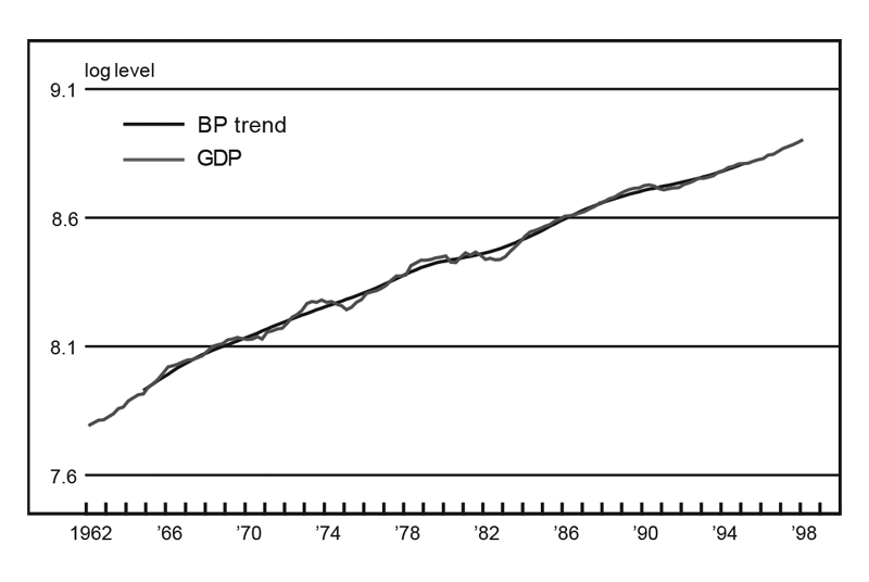
Source: Authors’ calculations based upon data from the U.S. Department of Commerce, Bureau of Economic Analysis, National Income and Product Account, 1962–98.
2. Trend component of GDP, UC method
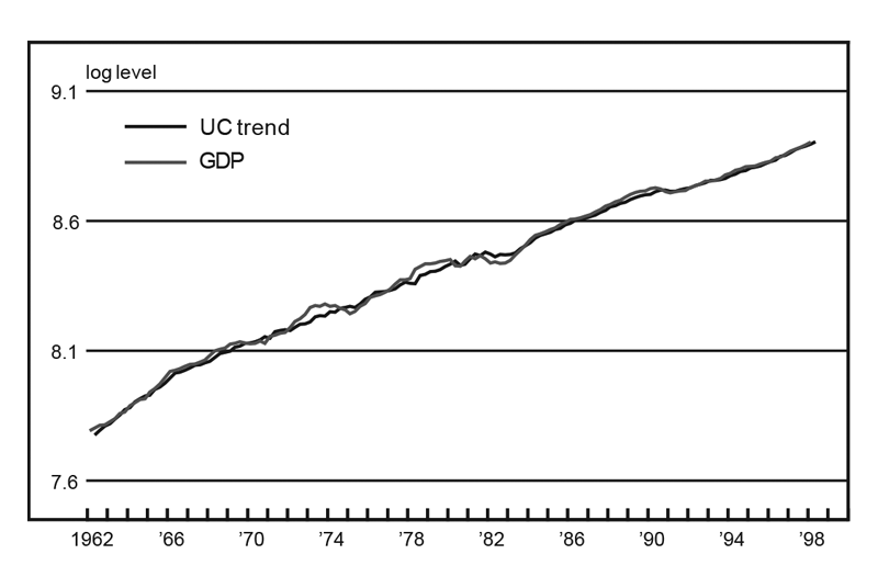
Source: Authors’ calculations based upon data from the U.S. Department of Commerce, Bureau of Economic Analysis, National Income and Product Accounts, 1962–98.
3. Cycle component of GDP
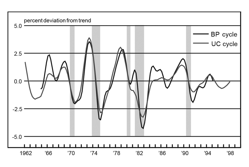
Source: Authors’ calculations based upon data from the U.S. Department of Commerce, Bureau of Economic Analysis, National Income and Product Accounts, 1962–98.
The advantage of the UC approach is that it generates an estimate of the underlying growth rate of the trend, which differs from the growth rate of the trend itself since the trend is subject to shocks that may permanently change its level while not changing its growth rate. Figure 4 plots the growth rate of the UC trend against the UC underlying trend growth rate and the BP trend growth rate. The BP trend growth rate and the UC underlying trend growth rate are considerably smoother than the UC trend growth rate. While the BP and UC underlying trend growth rates have been increasing over the 1990s, they have been doing so very slowly and are not any greater than they were in the 1980s. This evidence suggests that the high growth rates of U.S. output in the 1990s have not been due to an increase in the underlying trend growth rate but rather to temporary unobservable factors that have permanently raised the level of trend output.
4. Trend growth rate of GDP
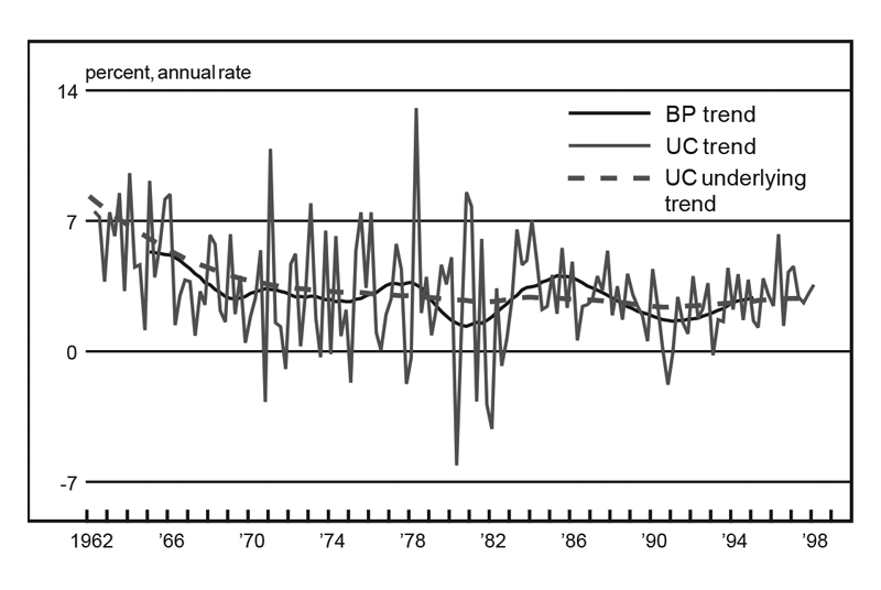
Source: Authors’ calculations based upon data from the U.S. Department of Commerce, Bureau of Economic Analysis, National Income and Product Accounts, 1962–98.
Conclusion
The popular press has hailed the dawn of a new paradigm in which the U.S. economy can expand at rates much greater than the past without igniting higher levels of price inflation. This concept is based on the belief that the U.S. experienced a structural change in the 1990s that raised its trend growth rate. Evidence presented here, which is based on one set of statistical tests, suggests that the underlying trend growth rate of U.S. output has not increased in the 1990s. In fact, our estimates suggest that the trend rate of growth has merely returned to the levels of the early 1980s. Overall, our statistical model suggests that the robust performance of the U.S. economy has been due to temporary factors that have permanently raised the level of U.S. production but have not changed the long-run growth rate of the U.S. economy.
Tracking Midwest manufacturing activity
Manufacturing output indexes (1992=100)
| July | Month ago | Year ago | |
|---|---|---|---|
| CFMMI | 121.2 | 124.5 | 123.0 |
| IP | 129.3 | 130.2 | 126.9 |
Motor vehicle production (millions, seasonally adj. annual rate)
| July | Month ago | Year ago | |
|---|---|---|---|
| Cars | 3.9 | 4.8 | 5.8 |
| Light trucks | 4.0 | 5.2 | 4.9 |
Purchasing managers' surveys: net % reporting production growth
| August | Month ago | Year ago | |
|---|---|---|---|
| MW | 59.2 | 52.0 | 59.9 |
| U.S. | 50.3 | 49.2 | 62.4 |
Manufacturing output indexes, 1992=100
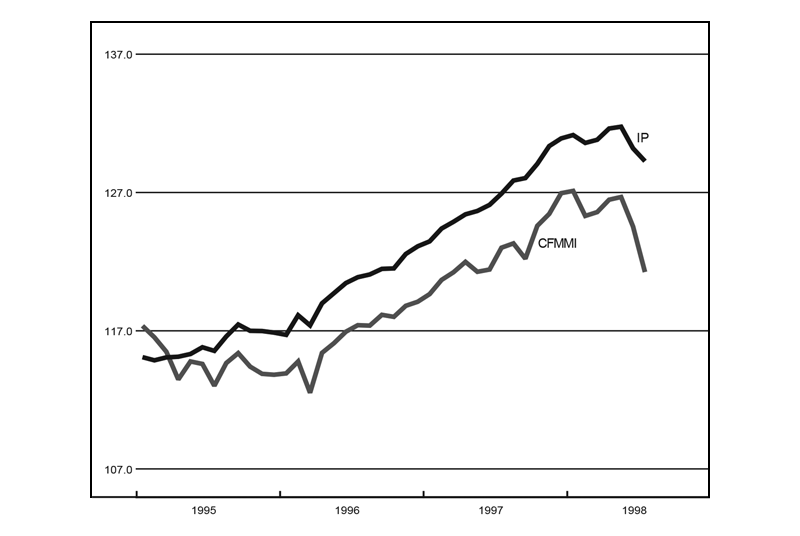
The Chicago Fed Midwest Manufacturing Index (CFMMI) decreased 2.6% in July following a revised decrease of 1.7% in June. The Federal Reserve Board’s Industrial Production Index (IP) for manufacturing declined 0.7% in July after declining 1.2% in June.
The Midwest purchasing managers’ composite index increased to 59.2% in August from 52.0% in July. Purchasing managers’ indexes increased in both Detroit and Milwaukee, but the index decreased in Chicago. Total light motor vehicle production decreased to 7.9 million units in July from 10 million units in June. Light truck production decreased to 4 million units in July from 5.2 million units in June and car production decreased to 3.9 million units from 4.8 million units during this period.
Notes
1 M. J. Mandel, 1997, “The new business cycle,” Business Week, March 31, pp. 58– 68, and S. B. Shepard, 1997, “The new economy: What it really means,” Business Week, November 17, pp. 38–40.
2 R. J. Barro and X. Sala-i-Martin, 1992, “Convergence,” Journal of Political Economy, Vol. 100, pp. 223–251.
3 S. T. Rebelo, 1991, “Long-run policy analysis and long-run growth,” Journal of Political Economy, Vol. 99, pp. 500–521.
4 R. G. King, C. I. Plosser, and S. T. Rebelo, 1988, “Production, growth and business cycles: The basic neoclassical model,” Journal of Monetary Economics, Vol. 21, pp. 195–232.
5 C. R. Nelson and C. I. Plosser, 1981, “Trends and random walks in macroeconomic time series: Some evidence and implications,” Journal of Monetary Economics, Vol. 10, pp. 139–162.
6 S. Beveridge and C. R. Nelson, 1981, “A new approach to decomposing economic time series into permanent and transitory components with particular attention to measurement of the ‘business cycle’,” Journal of Monetary Economics, Vol. 7, pp. 151–174.
7 R. Hodrick and E. Prescott, 1997, “Post- war U.S. business cycles: An empirical investigation,” Journal of Money, Credit, and Banking, Vol. 29, pp. 1–16.
8 M. Baxter and R. G. King, 1998, “Measuring business cycles: Approximate band-pass filters for economic time series,” International Economic Review, forthcoming.
9 M. W. Watson, 1986, “Univariate detrending methods with stochastic trends,” Journal of Monetary Economics, Vol. 18, pp. 49–75.
10 M. K. Burke and M. A. Kouparitsas, 1998, “Technical appendix: A new paradigm for the U.S. economy?” Federal Reserve Bank of Chicago, manuscript, forthcoming.
11 Baxter and King’s band-pass filter is approximated by a two-sided moving average, with a lag length of 12, so we lose the first and last 12 observations.


