

In recent weeks the country has begun to ease restrictions put in place to counter the Covid-19 pandemic. Consequently, it is important for policymakers and the public to understand the extent to which increasing levels of mobility among the population may lead to a rise in the spread of the disease.
In this Chicago Fed Letter, we consider two key questions. First, how long does it take for changes in mobility rates to be reflected in new cases and deaths? A sound understanding of the timing of these lags can enable policymakers to monitor the effects of changing policies more effectively. Second, how does a change in mobility affect the reproduction number, R, of the novel coronavirus 2019 (Covid-19)? The better we are able to understand this relationship, the more we will be able to fine-tune social distancing policies to prevent surges in Covid-19 cases.
Improving our understanding of the spread of the virus is important not only from a public health perspective but also from the standpoint of the economy. Future disease outbreaks may inhibit consumers and businesses from resuming activity either voluntarily or through the imposition of new government restrictions. Consequently, the Congressional Budget Office’s economic forecast for the second half of 2020 incorporates various possibilities regarding mobility and the rate of spread of Covid-19, including the risk of a resurgence later this year.1
The reproduction number, R
A key concept in epidemiology for understanding the rate of spread of any virus is the reproduction number, or R. This number indicates the average number of people a contagious person is likely to infect and can differ quite a bit across viruses. R is generally at its highest level at the beginning of an outbreak, before mitigation policies and behavioral changes start to reduce it. For policymakers, a critical value for R is 1. When R is above 1, more new people are infected than those that recover, and the number of infectious people will grow. In contrast, when R is less than 1, the number of infectious individuals will gradually decline. Therefore, one goal of policymakers is to try to keep R low. At the same time, there may be important societal and economic trade-offs, as the restrictions needed to keep R low could come at a very high cost. Several studies have tried to consider the optimal policies to balance these concerns.2 We do not take a stand on this issue. Our goal is simply to better understand the relationship between mobility and the spread of the disease in order to inform the policy discussion.
In an ideal world, if we knew exactly who was infected as soon as they were infected, we could estimate R by using data on infections. Unfortunately, such real-time information is not available. Instead, researchers typically estimate R by using observable measures, such as growth in new reported cases or deaths. However, these measures will only capture R with a significant lag of days or even weeks, depending on how exactly R is modeled.
There is a significant time lag between infection and when an actual case gets recorded (if a case gets recorded) for a few reasons. First, individuals infected with SARS-CoV-2, the strain of coronavirus that causes Covid-19, typically do not show symptoms for five to six days and could remain asymptomatic for up to 14 days. In fact, many infectious individuals experience no symptoms.3 Second, only those whose symptoms are relatively severe may seek medical care, adding further delay between the time of infection and the time of testing among those who are eventually tested. Third, there may be further delays in getting tested due to a lack of available tests and related equipment or other issues, and results can take up to a week as labs struggle to meet the surge in testing. Thus, observed cases may lag infections by many days or even weeks.
Furthermore, growth in cases may not provide an accurate view of R if those who are tested, and therefore recorded, are not representative of the actual infected population. On top of these issues is the likelihood that some of the lags, such as the time it takes to get tested and test turnaround delays, will change over the course of the pandemic, making it even more challenging to estimate the timing between mobility changes and disease spread.
An alternative to cases is to use observed deaths when calculating R. Due to the aforementioned issues with selective testing and associated timing problems, reported deaths are much more likely to be representative of the nature and timing of the spread of the virus.4 This is the approach taken by the Imperial College COVID-19 Response Team, one of the leading epidemiological research teams modeling the pandemic.5
For our analysis we estimate the daily growth in cases and deaths by state. A state enters our sample on the day in which Covid-19 cases or deaths are large enough to yield a reliable estimate.6 We use a weekly average of cases or deaths to reduce the noise in the estimates. The first state to enter our sample is Washington on March 9, 2020, followed by California on March 24, New York on March 25, and Louisiana and New Jersey on March 26. We also construct a population-weighted average of R for the entire country in order to summarize the spread of the virus at the national level.
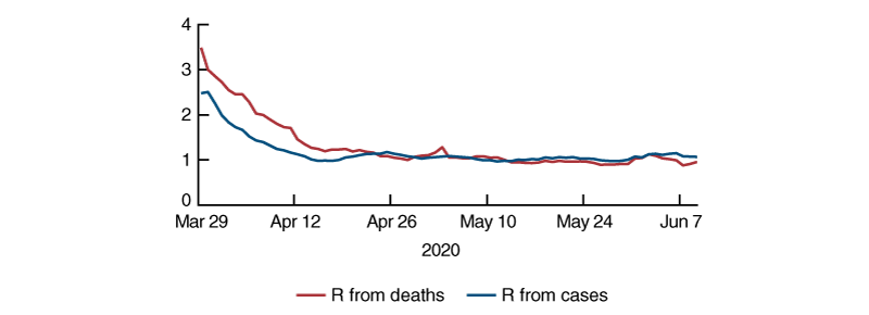
Figure 1 shows the national pattern in this proxy for R based on deaths and cases since March 29. At that point there were ten states contributing to the national average for R.7 As seen in the figure, both series declined sharply from late March to mid-April, and the decline in R from deaths lagged the decline in R from cases by about five to ten days. Since late April both proxy measures of R have been fairly stable and appear to be fluctuating around 1. Although there is uncertainty about its precise level, an R of around 1 is consistent with the plateau in the disease nationally, as cases have been steadily increasing by about 20,000 per day.
1. Estimates of R for the United States
Social distancing as measured by mobility
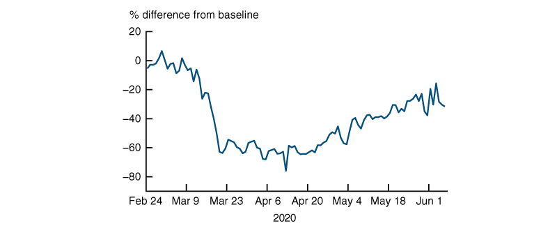
To capture social distancing, we use a mobility measure from Unacast derived from cell-phone usage that shows the percentage difference in the number of visits individuals have made to businesses considered nonessential relative to a pre-pandemic baseline level.8 Figure 2 shows the time pattern for the nation as a whole since late February. As concerns over the virus became widespread in mid-March, nonessential visits plunged, reaching a level of –60% below the baseline by March 20. From that time until late April/early May, when a few states began to reopen, this national mobility measure has stayed at or below –50%. For the first half of May, mobility averaged –45% and for the second half averaged –35%. The average measure for the first week of June was –28%.
2. National pattern of nonessential visits
How long does it take for mobility changes to be reflected in R?
In order to assess how long it takes for changes in mobility to be reflected in cases or deaths, we estimated the correlation between our two proxies for R shown in figure 1 with up to 30 daily lags of our social distancing measure shown in figure 2, using data through May 15.9 We plotted the correlations in figure 3. We find that the peak correlation between R estimated from cases and mobility is 15 days. The peak correlation from R estimated from deaths and mobility is 25 days. The peak correlations are indicated by the dots in the figure.10 There is also a considerable degree of heterogeneity in these estimates across states. We find a peak lag in cases, ranging from a low of ten days to a high of 27 days, and a peak lag in deaths ranging from 18 to 30 days.
3. Correlations between R based on cases or deaths and lags in mobility
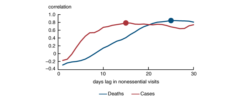
This suggests that the recent rise in mobility from –40% to –30%, as many states reopened in the second half of May, might not become apparent in recorded cases until mid-June and in deaths until late June. However, the actual magnitude of the rise in cases and deaths and their longer-term significance will depend on the level of R—in particular, whether it exceeds 1, and by how much.
What are the implications of this rise in mobility on disease spread?
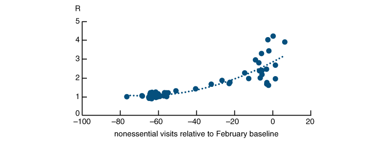
Now, we want to explore how a change in mobility will affect disease spread. Figure 4 shows a scatter plot of our national mobility measure on nonessential visits lagged by 25 days on the x-axis, against the national average of R based on the growth in deaths on the y-axis, through May 15. The relationship between R and mobility appears to be nonlinear. When mobility is very low, the relationship is fairly flat. An increase in mobility from –60% to –50% does not appear to increase R by very much and would likely keep R close to 1. In contrast, the recent increase in mobility from –40% to –30% may have driven R above 1 and to a level that could lead to more severe outbreaks. The dashed line shows the quadratic equation that best fits the data points.11
4. R versus mobility (25-day lag)
A very important caveat is that the implied relationship between mobility and R in figure 4 is based on the early months of the pandemic. It may well be the case that other behavioral changes, such as increased use of face masks and maintaining greater physical distance in daily interactions may alter this relationship. Furthermore, the actual level of R during the summer months may potentially be lower due to seasonal factors.12
We conducted some simulations using a standard SIR epidemiological model to gauge the effects of increased mobility.13 We assume that starting May 1, R is permanently lower by 10% due to behavioral changes, such as more widespread use of face masks. We also assume that R is lower by about 20% from May to August due to seasonal effects. Under these assumptions, we find that if mobility had stayed at its mid-May level of around –40% through the end of August, cumulative deaths would have been 144,000 by the end of August. An increase in mobility to –30% starting on June 1 leads cumulative deaths to be 232,000 by August 31, or an additional 88,000 deaths. In order to completely offset the increase in deaths from such an increase in mobility, we would have to assume a seasonal effect that lowers R by about 40%, which is at the very upper end of the range of estimates.14
A recent study by the Imperial College COVID-19 Response Team using a much more sophisticated model paints an even grimmer picture. Their model suggests that a 20% increase in mobility in the U.S. (the equivalent of an increase in mobility by our measure from –40% to –32%) could result in deaths that “exceed current cumulative deaths by greater than twofold, if the relationship between mobility and transmission remains unchanged.”15 At the time of their report, May 20, cumulative deaths were 91,664. This suggests that cumulative deaths due to such a rise in mobility could exceed 270,000 by late July.
We caution that these projections have a high degree of uncertainty and are also likely to change as individual behavior changes. If the disease spreads especially rapidly due to higher mobility and the negative health consequences become apparent, we would expect local authorities to impose or restore restrictions on mobility.
Conclusion
As the country has begun to reopen the economy and relax restrictions designed to counter the pandemic, there has been a notable increase in mobility as measured by daily nonessential visits. Based on the past relationship between mobility and cases and deaths, this increase in mobility may lead to increases in cases and deaths within two to four weeks and could raise the reproduction number, R, above 1, leading to an increase in the spread of the disease. Under some assumptions, and barring an especially large seasonal slowing of the virus, the corresponding rise in R due to increased mobility is projected to lead to a significant increase in the number of cumulative deaths by the end of the summer. Further increases in mobility could lead to even worse health consequences and might lead policymakers to consider implementing new restrictions on activity. If implemented, such restrictions would slow the economic recovery in the second half of the year.
Notes
1 Details available online.
2 See, for example, the following papers by Michael Greenstone and Vishan Nigam, 2020, “Does social distancing matter?,” University of Chicago, Becker Friedman Institute for Economics, working paper, No. 2020-26, March, Crossref; Daron Acemoglu, Victor Chernozhukov, Iván Werning, and Michael D. Whinston, 2020, “Optimal targeted lockdowns in a multi-group SIR model,” National Bureau of Economic Research, working paper, No. 27102, revised June 2020 (originally issued May 2020), Crossref; and Maryam Farboodi, Gregor Jarosch, and Robert Shimer, 2020, “Internal and external effects of social distancing in a pandemic,” National Bureau of Economic Research, working paper, No. 27059, April, Crossref.
3 It is not yet clear what fraction of cases show mild or no symptoms of the disease, with estimates varying from 5% to 80%. More information is available online.
4 However, there are concerns that not all Covid19-related deaths are classified as due to the virus, which could lead to underreporting of the true number of Covid-19 deaths. This is expected to improve over time as more deaths are reclassified.
5 See Imperial College London, COVID-19 Response Team, 2020, “State-level tracking of COVID-19 in the United States,” report, No. 23, London, UK, May 21. Crossref
6 We used thresholds of 15 deaths or 1,000 cases.
7 For the analysis below, we use all available values of R beginning March 9 for deaths and March 18 for cases.
8 Unacast, 2020 Unacast Social Distancing Dataset, available online, version from May 28. Nonessential business categories include many types of retail and services (shoe stores, clothing stores, spa/massage services), amenities (bars and restaurants, theaters, cinemas), and leisure facilities (bowling alleys, fitness centers).
9 We were inspired to do this exercise by a similar analysis done by Pat Bayer on a twitter thread on May 7, available online.
10 If we pool observations across states we obtain similar results. In this case, the mobility lag with the highest correlation with R based on cases is 19 days and the peak lag based on deaths is 25 days.
11 We obtain nearly identical results if we use a regression with pooled state data. If we also include state fixed effects in the regression, the shape of the quadratic curve is very similar but is shifted down, so that R is about 0.2 lower for each value of mobility.
12 Stephen M. Kissler, Christine Tedijanto, Edward Goldstein, Yonatan H. Grad, and Marc Lipsitch, 2020, “Projecting the transmission dynamics of SARS-CoV-2 through the postpandemic period,” Science, Vol. 368, No. 6493, May 22, pp. 860–868, Crossref, suggest that R could decline by as much as 40% in some places during the summer months.
13 The SIR model consists of three compartments: the number of individuals susceptible (S), the number infectious (I), and the number recovered, deceased, or immune (R). We use a model developed at the University of Basel (details available online).
14 See note 12.


