

The American Rescue Plan Act (ARP) signed into law on March 11, 2021, authorized approximately $1.9 trillion in federal government spending. ARP is widely expected to boost economic growth over the next two to three years—and significantly so early on. The upswing in growth is likely to increase resource pressures and therefore consumer price inflation as well. The potential for this channel to raise inflation substantially has attracted the attention of economic commentators, including Olivier Blanchard and Lawrence Summers.1 But the magnitudes and persistence of the possible increases in inflation are often left unsaid. In this article, we take a closer look into the effects ARP may have on inflation.
We quantify the potential effects through the lens of four Phillips curve (PC)2 models that relate inflation to expected inflation, resource pressures, and past inflation in different ways. In the three models grounded in data since 1990, the effects are generally modest and short-lived. The largest and most persistent effects come from a model grounded in data from the period 1960–90—when inflation was highly correlated with resource pressures, in contrast to the inflation dynamics of more recent times. While these older dynamics seem unlikely to reemerge, they are still a risk to the outlook.
Resource pressures may not be the only way ARP affects inflation. ARP is almost entirely deficit financed, so it will substantially add to the federal debt that is already high by historical standards. Such a large increase could trigger widespread concerns about the willingness of policymakers to increase taxes or reduce spending to contain the debt. This could boost inflation today if people come to widely believe a large fraction of the debt will be inflated away instead. We quantify the effect on inflation of such a change in beliefs using the model from Bianchi and Melosi (2017). We find the effects are small, as long as individuals do not believe the chances of inflating away the debt are high.
Four simple models of inflation
We assess the marginal effect of ARP on inflation via resource pressures using four simple models of inflation based on the PC described as follows.
Our first model is a version of the New Keynesian (NK) PC:
1) $\unicode{x03C0} _{t}^{q}=\text{ }\left( 1\text{ }-\unicode{x03B2} \right){{\unicode{x03C0} }^{*}}+\,\,\unicode{x03B2} {{E}_{t}}\unicode{x03C0} _{t+1}^{q}~-\,\unicode{x03BA} {{\hat{u}}_{t}}+{{\unicode{x03B5} }_{t}}.$
This model relates quarterly inflation measured at a quarterly rate at date t, $\unicode{x03C0} _{t}^{q}$, to the long-run inflation rate, $\unicode{x03C0}^*$; one-period-ahead expected inflation, $\unicode{x03B2} {{E}_{t}}\unicode{x03C0} _{^{t+1}}^{q}$; the unemployment gap, ${{\hat{u}}_{t}}$; and a disturbance term reflecting cost-push shocks or shocks to firms’ price markups, ${{\unicode{x03B5} }_{t}}$. The unemployment gap equals the difference between the actual unemployment rate and the unemployment rate consistent with no pressure on inflation, which is also called the “natural rate of unemployment.” The parameter $\unicode{x03B2} $ summarizes individuals’ discounting of the future. The slope of the PC $\unicode{x03BA} $ represents the sensitivity of inflation to ${{\hat{u}}_{t}}.$
We do not work with equation 1 directly because it involves inflation expectations, which we expect to change (at least in the short run) with the enactment of ARP. Instead we use the following equivalent representation:
${\unicode{x03C0} _{t}^{q}={{\unicode{x03C0} }^{*}}-\unicode{x03BA} {{E}_{t}}\sum\limits_{j=0}^{\infty }{{{\unicode{x03B2} }^{j}}}{{\hat{u}}_{t+j}}+{{e}_{t}}}$,
where ${{e}_{t}}={{E}_{t}}\sum{_{j=0}^{\infty }\,}{{\unicode{x03B2} }^{j}}{{\unicode{x03B5} }_{t+j}}.$ We assume that after some date $T$, unemployment has returned to its natural rate. Therefore,
2) $\unicode{x03C0} _{t}^{q}={{\unicode{x03C0} }^{*}}-\unicode{x03BA} {{E}_{t}}\sum\limits_{j=0}^{T}{{{\unicode{x03B2} }^{j}}{{{\hat{u}}}_{t+j}}+{{e}_{t}}.}$
Following Hazell et al. (2020), we suppose that
3) ${{E}_{t}}\sum\limits_{j=0}^{T}{{{\unicode{x03B2} }^{j}}{{{\hat{u}}}_{t+j}}}={{\unicode{x03C8} }_{0}}+{{\unicode{x03C8} }_{1}}{{\hat{u}}_{t}}+{{\unicode{0x03BD} }_{t}}.$
After substituting equation 3 into equation 2, the marginal effect of ARP on quarterly inflation measured at an annual rate, ${{\unicode{x03C0} }_{t}}$, is given by
4) $\Delta {{\unicode{x03C0} }_{t}}=\text{ }-4\text{ }\times \,\text{ }0.01\text{ }\times \text{ }6.16\left( \hat{u}_{t}^{ARP}-\hat{u}_{t}^{NOARP} \right)$,
where $\hat{u}_{t}^{NOARP}$ is the Congressional Budget Office (CBO) estimate of ${{\hat{u}}_{t}}$ without accounting for ARP and $\hat{u}_{t}^{ARP}$ corresponds to estimates of ${{\hat{u}}_{t}}$ discussed in the next section.3 Multiplying by the number 4 converts quarterly inflation into an annual rate; $\unicode{x03BA} \text{ }=\text{ }0.01$ and ${{\unicode{x03C8} }_{1}}=\text{ }6.16$, which are estimates from Hazell et al. (2020) using data (mostly) since 1990.
The next model, which we call the behavioral PC model, is designed to gauge the inflationary effects of ARP in the case when inflation dynamics are tied closely to those from the period 1960–90. This was a time of large swings in inflation and inflation expectations and pronounced co-movement of these variables with the unemployment gap, in comparison with more recent years. The behavioral PC model captures these dynamics by assuming that inflation expectations are backward-looking. We adopt a specification that yields a PC with “speed effects,” where inflation is related to the lagged level and contemporaneous change of the unemployment gap. This model is the same as equation 1 except we replace the expected inflation term with
\[{{E}_{t}}\unicode{x03C0} _{t+1}^{q}=0.89\unicode{x03C0} _{t-1}^{q}-0.11{{\hat{u}}_{t-1}}.\]
We leave $\unicode{x03BA} $ at 0.01 and set $\unicode{x03B2} $ at 0.976, and then calculate the marginal effect of ARP on inflation by solving equation 1 with these expectations recursively for the no-ARP and ARP paths of the unemployment gap, taking their difference, and converting the difference into an annual rate.4
Our third model is from Yellen (2015). This model is as follows:
5) ${{\unicode{x03C0} }_{t}}=0.41\unicode{x03C0} _{t}^{e}+0.36{{\unicode{x03C0} }_{t}}_{-1}+0.23{{\unicode{x03C0} }_{t}}_{-2}-0.08{{\hat{u}}_{t}}+0.57p_{t}^{ci}+{{v}_{t}}$,
where $\unicode{x03C0} _{t}^{e}$ is expected long-run inflation, $p_{t}^{ci}$ is a measure of inflation in the relative price of core imported goods, and ${{v}_{t}}$ is a disturbance term. Yellen (2015) estimates this model using the sample period 1990:Q1–2014:Q4. We assume $\unicode{x03C0} _{t}^{e}$, $p_{t}^{ci}$, and ${{v}_{t}}$ do not change with ARP, and then measure the marginal effect of ARP on inflation using the same method as for the behavioral PC model.
Our last model is a simple nonlinear version of Yellen’s model designed to capture the idea that at very low unemployment rates, resource pressures might have larger effects on inflation. In this case we suppose that the coefficient on the unemployment gap in equation 5 doubles when unemployment falls below 3.5%, the lowest rate achieved during the last expansion.
The models’ estimates of the inflationary effects of ARP due to resource pressures
We calculate $\hat{u}_{t}^{ARP}$ from estimates of the output gap using the Okun’s law relationship ${{\hat{u}}_{t}}=-0.5{{\hat{y}}_{t}}$, where ${{\hat{y}}_{t}}$ is the output gap, expressed as the percentage point deviation of gross domestic product (GDP) from its potential. Replacing ${{\hat{u}}_{t}}$ with $-0.5{{\hat{y}}_{t}}$ in equation 1 yields the PC from the canonical NK model. We consider three paths for GDP that are based on different assumptions about how fast the provisions of ARP are spent, as well as the impact of that spending on GDP.5 These assumptions are summarized as follows.
- No smoothing: This path uses estimates of the impact on GDP from the various provisions of ARP from Edelberg and Sheiner (2021), along with assumptions about when the provisions will be spent. This path takes on board Karger and Rajan’s (2020) finding that the CARES Act checks sent to households were spent quickly.
- Smoothing: This path also uses the impact estimates from Edelberg and Sheiner (2021), but allocates the spending more gradually over time.
- Conservative: This path assumes a pattern of spending similar to the no-smoothing case, but assumes smaller impact estimates.
We calculate output gaps from these GDP paths using the CBO’s projections of potential output. This means we assume that ARP has no impact on potential output.
Figure 1 shows the level of unemployment for the three ARP scenarios compared with the CBO estimate with no ARP. This CBO estimate falls gradually to about 4.5% by the end of the projection period. In all three ARP scenarios, unemployment falls faster and significantly lower than in the no-ARP scenario. Notably, unemployment in the smoothing case falls below the pre-pandemic level of 3.5% for three consecutive quarters, starting in 2021:Q4.
1. Unemployment in the three ARP scenarios and the no-ARP scenario
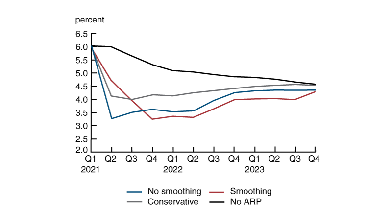
Sources: Authors’ calculations based on data from the Congressional Budget Office, Edelberg and Sheiner (2021), and Karger and McGranahan (see note 5).
The results presented in figure 2 are based on the NK PC. This figure and the next two show the additional inflation generated by ARP relative to a baseline path without ARP. This figure gives an indication of magnitudes one can expect from an empirically plausible PC slope, $\unicode{x03BA} =\text{ }0.01$. The boost to inflation in the no-smoothing case is quite large initially—70 basis points (bps) in 2021:Q2 and 55 bps in 2021:Q3—but the additional inflation dips below 50 bps in 2021:Q4 and falls steadily thereafter. With the smoothing case, the marginal inflation effect rises for three quarters, peaking at 53 bps in 2021:Q4, but falls below 50 bps in 2022:Q1 and ends up below 10 bps in 2023:Q4. The marginal effect on inflation in the conservative case never rises above 50 bps and falls quickly below 25 bps.
2. Additional inflation from ARP using the NK PC model
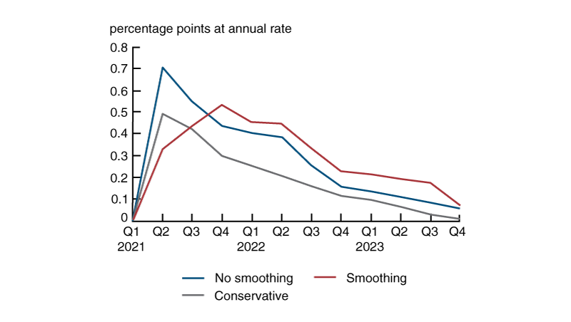
Sources: Authors’ calculations based on data from the Congressional Budget Office, Edelberg and Sheiner (2021), and Karger and McGranahan (see note 5).
The results shown in figure 3 are based on the behavioral PC. In the no-smoothing case, inflation is boosted about 100 bps by the end of 2022; in the smoothing case, the marginal inflation effect is similar, but the peak effects come a little later. The marginal effect on inflation in these two cases exceeds 50 bps toward the end of 2021 and stays above 50 bps for the remainder of the projection period. The inflation projections in the conservative case are also substantial. Inflation expectations in this model depend on lagged values of inflation and the unemployment gap and coefficient estimates based on data that include the 1960–90 period. This leads to long-lived changes in inflation expectations because inflation and unemployment moved together persistently in this earlier period.
3. Additional inflation from ARP using the behavioral PC model
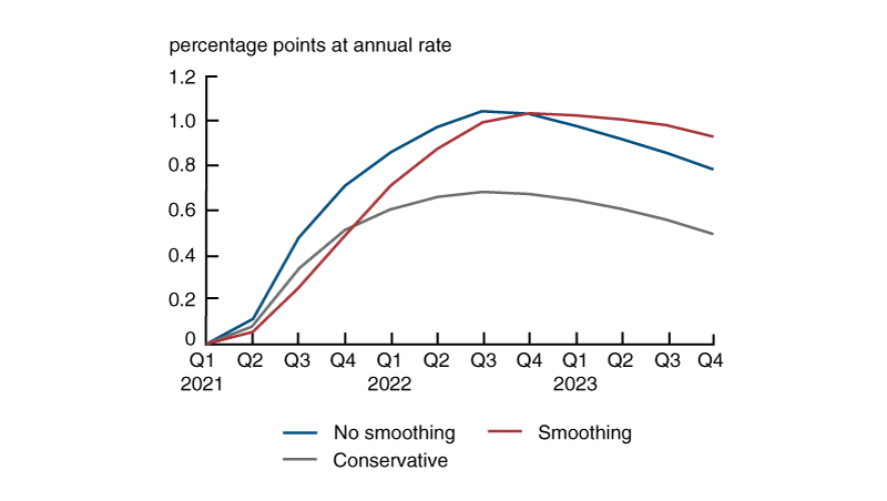
Sources: Authors’ calculations based on data from the Congressional Budget Office, Edelberg and Sheiner (2021), and Karger and McGranahan (see note 5).
Figure 4 shows the results from the linear Yellen (2015) model, along with one result from the nonlinear version of it. According to the linear model’s projections, the no-smoothing and smoothing paths of federal government spending raise inflation by up to nearly 30 bps by the middle of 2022 before declining gradually. In both of these cases, the marginal effect on inflation is near or above 20 bps for almost two years. Using the linear Yellen model, we find the boost to inflation in the conservative case is never more than 20 bps. Figure 4 also displays the marginal inflation path for the nonlinear Yellen model with the smoothing ${{\hat{u}}_{t}}$ path. As indicated in figure 1, the unemployment rate with smoothing dips below the 3.5% threshold in 2021:Q4 and stays below for another two quarters. The effect on inflation is relatively small, at most 15 bps additional inflation, on top of the effect from its linear-model-based counterpart.
4. Additional inflation from ARP using Yellen’s model
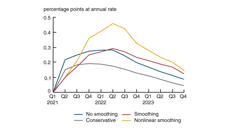
Sources: Authors’ calculations based on data from the Congressional Budget Office, Edelberg and Sheiner (2021), and Karger and McGranahan (see note 5).
Inflationary effects of ARP due to a change in beliefs about the federal debt
The previous analysis keeps long-run inflation expectations anchored; and the inflation effects of ARP, with the possible exception of those based on the behavioral PC model,6 seem consistent with this. Changes in long-term inflation expectations feed directly into current inflation. ARP is almost entirely deficit financed. With government debt already high, some may be concerned about a de-anchoring of inflation expectations due to growing beliefs that this debt will be inflated away. We now consider this possibility.
In NK models, the mere belief that policymakers may abandon the current mix of monetary and fiscal policies can bring about inflationary pressures. In theoretical terms the current policy mix (CPM) is represented by the combination of a fiscal policy rule that commits the fiscal authority to raise future primary surpluses to stabilize the debt-to-GDP ratio and a monetary policy rule in which the interest rate rises more than one for one with inflation. Abandoning the CPM means the economy switches to a regime in which the fiscal authority abandons its commitment to stabilize the debt and the monetary authority accommodates this change by responding less than one for one to inflation, thereby allowing inflation to rise.
To quantify the impact of a change in beliefs about a switch away from the CPM, we use the model from Bianchi and Melosi (2017). In this model, fearing the abandonment of the CPM, firms raise prices faster than they would otherwise because they face costs of adjusting prices and therefore wish to smooth out price changes. In our baseline case, we assume that costs of adjusting prices do not change across regimes.
We initialize the debt-to-GDP ratio to 110%, consistent with the federal debt held by the public at the end of 2020 and the size of ARP. All the other model variables are assumed to start from their steady-state values. The model evolves deterministically for ten years, and policymakers stay with the CPM. However, the private sector believes that policymakers might switch away from the CPM with some fixed probability in the coming years. If the CPM is abandoned, the private sector expects that the new regime will stay in place forever after, implying that inflation must rise to stabilize the existing debt-to-GDP ratio around its long-run level. This long-run ratio is assumed to equal average U.S. federal debt held by the public as a fraction of GDP from 1960 through 2019—i.e., 40%. The slope of the model’s PC is set to 0.01 as in the previous section. The model’s other parameters are calibrated following Bianchi and Melosi (2017).7
The blue bars in figure 5 show the contribution of the fiscal imbalance to average inflation over the next ten years (after the enactment of ARP) for various probabilities held by the public that policymakers will abandon the CPM over the next five years. If the private sector believes there is a 5% probability of abandoning the CPM permanently over the next five years, which seems high, inflation would rise by only 54 bps on average over the next ten years. However, the contribution to average inflation grows substantially as the probability increases. This suggests that, according to the model, the high debt represents a macroeconomic vulnerability, in that if there is a sharp change in beliefs about debt stabilization, it could have a substantial impact on inflation.
5. Average contribution to inflation over the next ten years due to changes in beliefs about federal debt stabilization
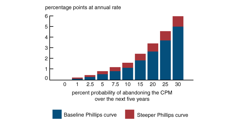
Source: Authors’ calculations.
Given that the public expects inflation will be higher, price-setting behavior might change as well. The red bars in figure 5 show the effect of lowering the costs of price adjustment so that the slope of the PC doubles in the new regime. This increases actual and expected inflation under the CPM because the private sector expects inflation to be even higher if the regime switches. However, for low probabilities of switching, the effect remains quite modest.
We view the bars in figure 5 as upper bounds on the model’s effects of a change in beliefs about debt stabilization because we set the long-run level around which the debt-to-GDP ratio must be stabilized to its average for the period 1960–2019. Greater demand for U.S. debt compared with most other forms of debt during this period due to the so-called global saving glut (GSG)8 could make it possible to sustain a higher level of debt. If we raise the long-run debt-to-GDP ratio, the bars in figure 5 become shorter. Furthermore, the private sector could expect policymakers to use a mix of tools—not just inflation—to stabilize the debt. If the private sector expects that only a fraction of the debt will be inflated away, the bars in figure 5 will be shorter as well.
Conclusion
We have explored alternative scenarios for the potential inflationary effects of ARP through resource pressures generated by new federal spending and its possible impact on the public’s beliefs about the federal debt. With most of our models, we find that resource pressures generally have small and transitory effects on inflation. However, one model grounded in data before 1990 shows there can be larger and more persistent effects. We also find that if ARP generates a change in beliefs about the likelihood that a portion of the federal debt will be inflated away, the effects on inflation will be small as long as individuals do not believe the chances of a switch in policy regime are high.
Notes
1 Blanchard (2021) and Summers (2021a, 2021b).
2 The Phillips curve was named after William Phillips (1958), who noted an inverse relationship between the unemployment level and money wage changes (or wage inflation) in the British economy. Since the publication of his 1958 paper, the relationship has been more broadly extended to price inflation.
3 All the CBO data we use are from their February 2021 release, available online.
4 We estimate the coefficients of the backward-looking expectations by regressing $\unicode{x03C0} _{t+1}^{q}$ on $\unicode{x03C0} _{t-1}^{q}$ and ${{\hat{u}}_{t-1}}$ for the sample period 1959:Q1–2019:Q4, using quarterly core inflation (which removes more volatile food and energy prices) according to the Personal Consumption Expenditures Price Index from the U.S. Bureau of Economic Analysis and the CBO’s ${{\hat{u}}_{t}}.$
5 We thank Ezra Karger and Leslie McGranahan for constructing these alternative GDP paths.
6 This statement is based on stepping outside of the model and considering the possibility that persistently higher inflation could be a source of de-anchoring.
7 Unlike in their model, we include lagged inflation in the PC and a feature called “external habit” that increases households’ incentive to smooth consumption. We use the corresponding parameters estimated in Campbell et al. (2017).
8 For a recent retrospective on the GSG hypothesis, see Barsky and Easton (2021).
References
Barsky, Robert, and Matthew Easton, 2021, “The global saving glut and the fall in U.S. real interest rates: A 15-year retrospective,” Economic Perspectives, Federal Reserve Bank of Chicago, No. 1. Crossref
Bianchi, Francesco, and Leonardo Melosi, 2017, “Escaping the Great Recession,” American Economic Review, Vol. 107, No. 4, April, pp. 1030–1058. Crossref
Blanchard, Olivier, 2021, “In defense of concerns over the $1.9 trillion relief plan,” RealTime Economic Issues Watch, Peterson Institute for International Economics, blog, February 18, available online.
Campbell, Jeffrey R., Jonas D. M. Fisher, Alejandro Justiniano, and Leonardo Melosi, 2017, “Forward guidance and macroeconomic outcomes since the financial crisis,” in NBER Macroeconomics Annual 2016, Martin Eichenbaum, Erik Hurst, and Jonathan A. Parker (eds.), Vol. 31, Chicago: University of Chicago Press, pp. 283–357. Crossref
Edelberg, Wendy, and Louise Sheiner, 2021, “The macroeconomic implications of Biden’s $1.9 trillion fiscal package,” The Hamilton Project, Brookings Institution, blog post, January 28, available online.
Hazell, Jonathon, Juan Herreño, Emi Nakamura, and Jón Steinsson, 2020, “The slope of the Phillips curve: Evidence from U.S. states,” National Bureau of Economic Research, working paper, No. 28005, revised November. Crossref
Karger, Ezra, and Aastha Rajan, 2020, “Heterogeneity in the marginal propensity to consume: Evidence from Covid-19 stimulus payments,” Federal Reserve Bank of Chicago, working paper, No. 2020-15, revised October 8. Crossref
Phillips, A. W., 1958, “The relation between unemployment and the rate of change of money wage rates in the United Kingdom, 1861–1957,” Economica, Vol. 25, No. 100, November, pp. 283–299. Crossref
Summers, Lawrence H., 2021a, “My column on the stimulus sparked a lot of questions. Here are my answers.,” Opinions, Washington Post, February 7, available online.
Summers, Lawrence H., 2021b, “The Biden stimulus is admirably ambitious. But it brings some big risks, too.,” Opinions, Washington Post, February 4, available online.
Yellen, Janet L., 2015, “Inflation dynamics and monetary policy,” speech by the Board of Governors of the Federal Reserve System Chair at the Philip Gamble Memorial Lecture, University of Massachusetts Amherst, September 24, available online.


