

A half century after gold ceased to play a significant formal role in the international monetary system, it still captures a great deal of attention in the financial press and the popular imagination. Yet there has been very little scrutiny of the primary factors determining the price of gold since its dollar price was first allowed to vary freely in 1971.1 In this article, we attempt to fill in that gap by highlighting three considerations that are commonly cited as drivers of gold prices: inflationary expectations, real interest rates, and pessimism about future macroeconomic conditions.
Our empirical results in this Chicago Fed Letter are organized around three claims—namely, that gold is a hedge against inflation, gold is sensitive to expected long-term real interest rates, and gold is regarded as protective against “bad economic times.”
Gold is a hedge against inflation. A rise in inflation or inflationary expectations increases investors’ interest in purchasing gold and, therefore, drives up its price; in contrast, disinflation or a drop in inflationary expectations does the opposite. We will measure the “inflation hedge” motive for holding gold with PTR—which is the mnemonic for the survey-based ten-year inflation expectation that is provided by the Board of Governors of the Federal Reserve System; PTR has in recent years coincided with the ten-year inflation projection of the Survey of Professional Forecasters (SPF) conducted by the Federal Reserve Bank of Philadelphia.2 The notion that gold can be identified with an inflation protection motive is of course connected with the fact that, in contrast to fiat money, gold is in nearly fixed supply. But this property of gold is shared by many other commodities. The special status accorded gold may be a relic of the gold standard era, or it may even reflect a belief on the part of a subset of investors that there is a positive probability that the world will at some point return to a gold standard. Figure 1 shows how the real price of gold and the long-term inflation expectation have evolved over time. The measure of the real gold price is the London PM fixing price for gold (from the London Bullion Market Association) in U.S. dollars per ounce deflated by the U.S. Consumer Price Index, or CPI (from the U.S. Bureau of Labor Statistics), plotted on a log scale; and the measure of expected inflation over the next ten years is PTR. From 1971 to around 2000, the real gold price and the long-term inflation expectation tend to move together. A sharp uptick in inflation expectations during the period 1971–80 coincides with a dramatic run-up in gold prices. Gold prices fell dramatically during the Volcker disinflation of 1980–83.3 Over the period 1983–2000, the steady downward march of expected long-term inflation following the Volcker disinflation period coincides with the decrease in the real gold price. Since 2000, however, the long-term inflation expectation has deviated relatively little from 2%, whereas the real gold price has increased more than fivefold. The role of expected inflation in this later period seems to have given way to that of the real interest rate—our second key driver of the gold price—which we discuss next.
1. Real price of gold and ten-year inflation expectation, 1971:Q1–2021:Q1

Sources: Authors’ calculations based on data from the London Bullion Market Association and Board of Governors of the Federal Reserve System.
Gold is sensitive to expected long-term real interest rates. Given that gold is a long-duration durable asset with a relatively stable dividend yield, its price is expected to have a strong inverse relationship with the long-term real interest rate. A rise in expected real rates, all else being equal, should drive down the price of gold.4 Figure 2 shows the real gold price (the U.S. dollar price per ounce deflated by the CPI, once again on a log scale), along with the real ten-year U.S. Treasury yield (the nominal yield on ten-year Treasury securities minus PTR). The predicted negative co-movement of the real interest rate and the real gold price does not show up in these data before 2001.5 By contrast, between 2001 and 2012, the long-term real interest rate fell some 400 basis points, accompanied by an over fivefold rise in the real gold price.
2. Real price of gold and real ten-year U.S. Treasury yield, 1971:Q1–2021:Q1

Sources: Authors’ calculations based on data from the London Bullion Market Association and Board of Governors of the Federal Reserve System.
Gold is regarded as protective against “bad economic times.” We test for this factor’s importance by using the Surveys of Consumers conducted by the University of Michigan (Michigan survey); one of the key survey questions is the following: “Looking ahead, which would you say is more likely—that in the country as a whole we’ll have continuous good times during the next 5 years or so, or that we will have periods of widespread unemployment or depression, or what?”6 We use as our measure the fraction of pessimistic responses to this question, and refer to it as “pessimistic expectations” in our analysis. Figure 3 shows the log real gold price along with the fraction of respondents to the Michigan survey who expect the next five years to be characterized by mostly bad times; there is considerable positive correlation between these two variables over our sample period.
3. Real price of gold and pessimistic expectations for the U.S. macroeconomy, 1971:Q1–2021:Q1
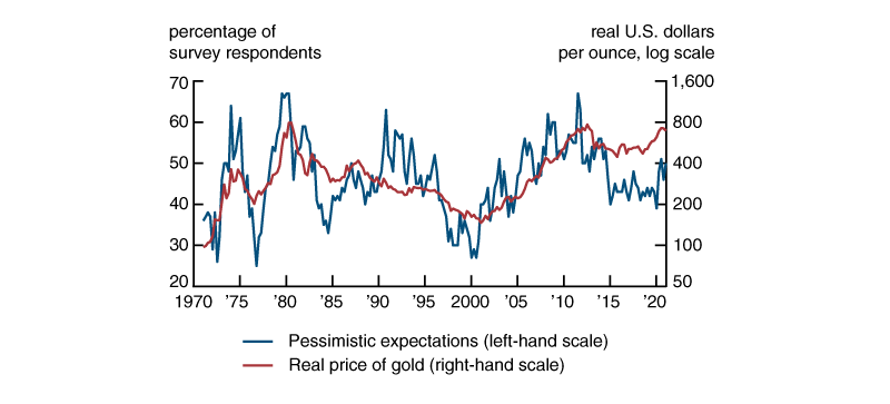
Sources: Authors’ calculations based on data from the London Bullion Market Association and University of Michigan, Surveys of Consumers.
Multiple regressions
Comparing figures 1–3 reveals that the key factors driving gold price variation often move together. For example, the rather steady rise in pessimistic expectations (figure 3) between 2001 and 2012 matches a persistently falling real interest rate over the same period (figure 2). To disentangle the roles of the various factors over time, we perform multiple regressions.7 Our regressions provide a simple econometric evaluation of the contribution of our three key factors to the time-series variation in the real gold price over the period 1971–2021. In addition, we show that one additional factor proxied by real world or U.S. gross domestic product (GDP) plays an important role in accounting for the long-run trend in gold prices.
We begin with regressions that explain the association between the average annual log level of real gold prices and four variables, also at the average annual level: 1) the real U.S. dollar value of world GDP provided by the World Bank, 2) the expected ten-year real interest rate computed as the nominal ten-year U.S. Treasury yield minus the Federal Reserve Board’s PTR, 3) PTR itself, and 4) the fraction of the Michigan survey’s participants expecting largely bad economic times over the next five years (i.e., the pessimistic expectations variable). These regressions highlight the sources of longer-term variation in the level of real gold prices over the past half century (see figure 4). Although we find this exercise to be the most revealing about the basic historical movements of gold prices, the sample is not large and, more importantly, the degree of persistence in the error term is substantial, as indicated by the relatively low Durbin–Watson statistic of 0.98.8 The second regression exercise (whose results are reported in figure 5) uses essentially the same variables; but instead of looking at levels, it looks at the relationship between the log change in the real gold price and news about the explanatory variables using quarterly data. Finally, we conduct a limited investigation using daily data (whose regression results are reported in figure 6). The precise variables discussed here are not available at the daily frequency. However, we can investigate the roles of expected real rates and expected inflation using daily data on Treasury Inflation-Protected Securities (TIPS) and break-even inflation rates9 relative to nominal Treasury yields. In these three exercises, as in all regressions on nonexperimental data, it is important to repeat the usual caveat that the statistical analysis reveals correlations in the data, but does not in itself establish causality. The extent to which such regressions go beyond mere association depends on the “reasonableness” of the coefficients (see note 7) and, in short, the ability to “tell the story” that goes with the regressions.
Figure 4 shows the annual regression results. The real world GDP measure, which comes in highly significantly, reflects the fact that the demand for the services of gold and the demand for other goods increase together, approximately one-for-one in percentage terms. The estimated coefficient on the ten-year Treasury yield minus PTR indicates that a percentage point rise in the long-term real interest rate lowers the real gold price by 13.1%. PTR has an additional effect over and above its presence as a component of the real rate—and indeed this is far stronger quantitatively. Given the long-term real interest rate, an extra percentage point of ten-year expected inflation raises the real gold price by a hefty 37%—well in line with the long-held “inflation hedge” view. Finally, evaluated at the mean of 0.46, a one standard deviation increase in the fraction of pessimistic survey respondents (8.1 percentage points) raises the gold price by 9.7%.
4. Factors influencing annual real gold prices, 1971–2019
| Log (real gold price) |
|
|---|---|
| Log (real world GDP) | 1.125* (0.105) |
| Ten-year Treasury yield – PTR | –0.131* (0.022) |
| PTR | 0.365* (0.033) |
| Pessimistic expectations | 0.012* (0.004) |
| Constant | –35.588* (3.329) |
| R-squared | 0.87 |
| Durbin–Watson statistic | 0.98 |
Notes: Standard errors are in parentheses. The standard errors have been corrected for serial correlation using the Newey–West method. See the text for details on the real gold price, real world gross domestic product (GDP), real ten-year Treasury yield, PTR (a measure of the ten-year inflation expectation), and pessimistic expectations (based on University of Michigan survey results).
Sources: Authors’ calculations based on data from the London Bullion Market Association, World Bank, Board of Governors of the Federal Reserve System, and University of Michigan, Surveys of Consumers.
For figure 5, we shift our focus to quarterly data. Here the conceptual experiment is to ask how news about the explanatory variables is reflected in contemporaneous changes in the log real gold price. In addition to the markedly reduced concern about serially correlated errors, this has somewhat more of a causal feel than the levels regression in figure 4, although the coherent story told by the levels regression gives it more economic credibility than it would have on its purely econometric merits alone. For the exercise whose results are reported in figure 5, we replace the world output series with real U.S. GDP, in logs, given that our world GDP series is only available annually. The news variables are constructed by running four predictive regressions—collectively called a vector autoregression (VAR)—on the explanatory variables; the innovations from this VAR constitute the news (or surprise) component of the key explanatory variables.10 A 1% innovation in log real U.S. GDP is associated with a rise in the real gold price of 0.4%, substantially lower than the 1.1% value in the first row in figure 4, although in figure 5 the coefficient is very imprecisely estimated (indeed not statistically significant). A 1 percentage point innovation in the expected ten-year real interest rate (the nominal yield on ten-year Treasury securities minus PTR) is associated with a 3.4% reduction in real gold prices. In striking contrast with the result in figure 4, after accounting for the real interest rate, innovations in PTR play no significant role in the gold price. The coefficient on innovations in the pessimistic expectations variable appears small, but this is deceptive because of the large units in which the pessimistic expectations variable is measured, as well as the large variation in this variable over time. A 10 percentage point innovation in the fraction of survey participants who expect the next five years to constitute mostly bad times raises the real gold price by 5%. Because the pessimistic expectations variable repeatedly reaches lows of about 30% and highs of 60%, over the entire sample it drives substantial fluctuations in the real gold price.
5. Factors influencing changes in quarterly real gold prices, 1971:Q1–2021:Q1
| ∆ Log (real gold price) |
|
|---|---|
| Innovations in log real U.S. GDP | 0.395 (0.625) |
| Innovations in (ten-year Treasury yield – PTR) | –0.034* (0.011) |
| Innovations in PTR | 0.010 (0.044) |
| Innovations in pessimistic expectations | 0.005* (0.001) |
| Constant | 0.010 (0.006) |
| R-squared | 0.12 |
| Durbin–Watson statistic | 1.91 |
Notes: Standard errors are in parentheses. See the text for details on the real gold price, as well as the VAR (vector autoregression) innovations in log real U.S. gross domestic product (GDP), real ten-year Treasury yield, PTR (a measure of the ten-year inflation expectation), and pessimistic expectations (based on University of Michigan survey results).
Sources: Authors’ calculations based on data from the London Bullion Market Association, U.S. Bureau of Economic Analysis, Board of Governors of the Federal Reserve System, and University of Michigan, Surveys of Consumers.
Finally, we do a limited exercise using daily data and report the results in figure 6. Because the CPI is published only monthly, the dependent variable is the daily change in the nominal gold price. This is less problematic than it may at first appear because if we could observe daily changes in the overall price index, they would be at least two orders of magnitude less than the corresponding changes in the highly volatile nominal gold price. Of the independent variables we study in this article, only measures of the real yield on long-term Treasury securities and expected long-term inflation—in this case taken from the TIPS market—are available at a daily frequency. However, we regard this as useful for two reasons. First, the regression is run on the daily differences in the log nominal gold price; innovations in real GDP or pessimistic views on the next five years are likely to be essentially constant at this frequency. Second, the roles of expected real interest rates and inflation have been our most central theme (as evidenced by the coefficients in figures 4 and 5), and we have the data to obtain at least some evidence on these at the daily frequency. Since the variables are in differences, which are quite noisy, the R-squared, which measures the fraction of the variance of the dependent variable that is explained by the regression, is only 0.012. Yet, there are valuable lessons in this exercise. First, the negative effect of the real interest rate on the gold price—the proposition that comes most directly from economic theory—is once again confirmed. Hence, it has been shown to hold in annual levels, quarterly innovations, and daily differences. Second, the observation that the inflation effect is quantitatively much larger than the real interest rate effect holds here, as was the case in the levels regression of figure 4, though contrary to the innovations regression of figure 5.
6. Factors influencing changes in daily nominal gold prices, January 7, 2003–February 12, 2021
| ∆ Log (nominal gold price) |
|
|---|---|
| ∆ TIPS yield | –0.011* (0.004) |
| ∆ Break-even inflation rate | 0.027* (0.005) |
| Constant | –1.71E-05 (2E-04) |
| R-squared | 0.012 |
| Durbin–Watson statistic | 2.11 |
Notes: Standard errors are in parentheses. TIPS means Treasury Inflation-Protected Securities. See the text for details on the break-even inflation rate.
Sources: Authors’ calculations based on data from the London Buillon Market Association and Board of Governors of the Federal Reserve System.
Conclusion
We have investigated several hypotheses about the determinants of gold prices—in annual levels data, quarterly data in innovations form, and daily data in differences. The negative effect of real interest rates on gold prices predicted by theory holds in all three contexts. Two of the three specifications (the quarterly innovations specification being the exception) support the notion that gold is an inflation hedge and that this effect is quantitatively larger than the real interest rate effect. The two specifications that can be used to evaluate the proposition that gold prices also reflect protection against bad economic times are highly supportive of it. In the early part of the sample, variation in inflation or inflationary expectations was the single most important consideration for the real price of gold. From 2001 on, however, long-term real interest rates and pessimism about future economic activity appear as the dominant factors. While disinflation since 2001 might have been expected to result in low gold prices, any effect of low inflation was more than compensated for by unprecedentedly low long-term real interest rates and by pessimism about future economic activity.
Notes
1 The Bretton Woods system—which pegged the U.S. dollar price of gold and, for the most part, fixed ratios between gold and the other main currencies—collapsed in stages because of inherent contradictions in the design of the system. In 1971, the U.S. Gold Window was closed and the fixed price of gold vis-à-vis the dollar ended. We thus begin our sample in 1971. For a full explanation, see Michael Bordo, 2017, “The operation and demise of the Bretton Woods system: 1958 to 1971,” VoxEU.org, April 23, available online.
2 PTR is from the Federal Reserve Board’s FRB/US model’s database; see note 4 of John M. Roberts, 2018, “An estimate of the long-term neutral rate of interest,” FEDS Notes, Board of Governors of the Federal Reserve System, September 5. Crossref
3 Further details on the U.S. disinflation period of the early 1980s associated with former Federal Reserve Chair Paul Volcker are in Michael D. Bordo and Athanasios Orphanides, 2013, “Introduction,” in The Great Inflation: The Rebirth of Modern Central Banking, Michael D. Bordo and Athanasios Orphanides (eds.), Chicago: University of Chicago Press, pp. 1–22, available online.
4 This idea manifests itself in at least two ways. First, for the owner of a gold mine to be indifferent between keeping gold in the ground on the one hand and mining it and investing the proceeds in financial assets on the other, the price must be expected to rise at the rate of interest. Given an appropriate terminal condition, the higher the expected real interest rate, the lower the initial price would have to be. A second approach would be to imagine that gold provides some service flow (e.g., its value as jewelry). The present value of that “dividend stream” depends inversely on the real interest rate.
5 This is in contradiction with Barsky and Summers (1988), who found a strong negative correlation between the real gold price and their measure of the real interest rate, particularly over the period 1973–82; rather than using survey-based inflation expectations, they used a statistical model of inflation that was more sensitive to current inflation and thus provided a quite different series for expected long-term inflation. See Robert B. Barsky and Lawrence H. Summers, 1988, “Gibson’s paradox and the gold standard,” Journal of Political Economy, Vol. 96, No. 3, pp. 528–550. Crossref
6 The full Michigan survey questionnaire is available online.
7 Multiple regressions are statistical exercises estimating the effects of several independent variables on a dependent variable. Each regression coefficient represents the mean change in the dependent variable for a one-unit change in the independent variable while holding constant the other independent variables.
8 The Durbin–Watson statistic—which measures the degree of persistence or serial correlation in the residuals (differences between the observed values and the values predicted by the regression model)—takes on a value close to 2 in the ideal case where the residuals are serially uncorrelated. A value close to zero indicates that the errors are so persistent that the regression is “spurious” (uninterpretable and effectively meaningless). The Durbin–Watson statistic of 0.98 in the current regression exceeds the level at which the regression would be regarded as spurious, but raises some questions about how well specified the regression is—an issue largely addressed by the innovations formulation in figure 5. In addition, the standard errors of the coefficients in figure 4 have been corrected for serial correlation as indicated in that figure.
9 The TIPS yield, as noted on the Federal Reserve Board’s website, is a real rate. The break-even inflation rate is the one that would in principle make a risk-neutral investor indifferent between holding a nominal Treasury security and a TIPS of the same duration. It is often regarded as a measure of inflationary expectations at the relevant horizon.
10 A VAR is a statistical model used to capture the dynamic relationship between two or more time-series variables; in a VAR, each variable is a linear function of past lags of itself and past lags of the other variable(s). In a VAR context, an innovation is the difference between the observed value of a variable at a particular point in time and the optimal forecast of that value based on information available before that point in time.


