

Introduction and summary
Forecasting inflation accurately is critical for making many policy decisions. A key modeling choice that economists and policymakers face when forecasting inflation is whether to forecast aggregate inflation directly or its individual components first and then aggregate the results. Another important modeling decision is whether or not to group certain components (for instance, core and noncore components1) and then model them separately. In this article, we present a new disaggregated approach to forecasting inflation. Our focus is on inflation as measured by the Personal Consumption Expenditures (PCE) Price Index from the U.S. Bureau of Economic Analysis (BEA). We developed this new approach primarily because of the widespread heterogeneity evident in the dynamics of inflation both across its components and over time. In what follows, we begin by documenting this heterogeneity in PCE inflation. We then discuss the BEA data we used in our research and explain our method for microforecasting inflation in the PCE components—which we subsequently aggregate to derive a total PCE inflation forecast. Finally, we compare the forecasting accuracy of our novel approach and other methods, including those that forecast aggregate inflation directly. We find that over our sample period and other subperiods, the forecasts produced by our method are more accurate than those produced by the alternative approaches considered here.
Motivation for a new approach to forecasting inflation
Consider the dynamics of inflation as captured by the persistence of monthly inflation—or its tendency to remain near its most recent values. Figure 1 plots the quantiles of the distribution of monthly inflation persistence across the components of PCE inflation (estimated as described in the next section) as a function of time. This figure shows substantial heterogeneity in PCE inflation persistence, both across its components and over time. In this graph, we specifically track the inflation persistence of the eggs and fresh milk components of the PCE index. Their persistence varies widely over time, even switching between positive and negative readings during different periods. Given that eggs and fresh milk are both foods subsumed under the single broader PCE category of milk, dairy products, and eggs, these two components might be expected to have similar inflation dynamics; however, this is clearly not the case. The graph also highlights a pattern that we found occurs more broadly: A specific component doesn’t necessarily fall in the same quantile of the distribution of persistence at different points in time.
1. Heterogeneous persistence of inflation in components of the Personal Consumption Expenditures (PCE) Price Index
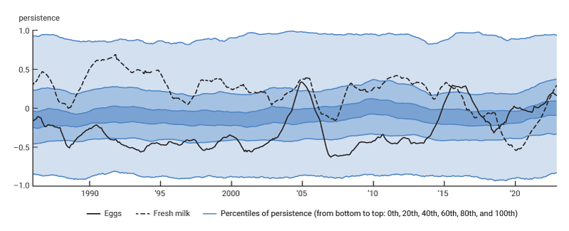
Source: Authors’ calculations based on data from the U.S. Bureau of Economic Analysis, National Income and Product Accounts of the United States, from Haver Analytics.
One implication of figure 1 is that we cannot treat persistence as a fixed characteristic of inflation. Also, it is clear that any grouping of inflation components based on invariant characteristics (for instance, core and noncore or durables, nondurables, and services) would mix very different inflation dynamics and mask the true extent of the heterogeneity. These findings have motivated us to focus on a novel disaggregated approach to forecasting inflation—one that takes into account the heterogeneous dynamics of inflation across components and over time.
Forecasting heterogeneous inflation components
In this section, we describe the BEA data we used to develop our new method for forecasting PCE inflation. We then explain our new methodology for microforecasting inflation in the PCE components to eventually get an aggregate PCE inflation forecast.
Data
We use publicly available price and quantity data released by the U.S. Bureau of Economic Analysis. These BEA data are from the underlying detail tables for prices and expenditures of the Personal Consumption Expenditures Price Index (tables 2.4.4U and 2.4.5U, respectively) in the National Income and Product Accounts of the United States (NIPAs).
The BEA constructs different levels of data that are disaggregated further with each level. The degree of the BEA’s disaggregation depends on the category of the product. For this article, we use the disaggregated components of the PCE index that are used by the Dallas Fed to compute their trimmed mean PCE rate. All of the components are from series that are at least at the fourth level of disaggregation. For example, goods (level 1) subsume durable goods (level 2), which subsume recreational goods and vehicles (level 3), which in turn subsume recreational books (level 4). The vast majority of the components are at level 5 or higher of disaggregation. By using the same set of PCE components as the Dallas Fed, we have 177 categories to work with.2 We eliminated a few series that were extremely volatile (namely, net motor vehicle and other transportation insurance, net health insurance, and life insurance) or had more than ten consecutive months of zero inflation (namely, motorcycles and employment agency services), which left us with 172 inflation components (see the appendix for the complete list of PCE components we used for this article).
Forecasting methodology
We model inflation in each PCE component as a first-order autoregression, or AR(1). We focus on a simple model for illustrative purposes; however, the approach described here can be applied more generally to any model with individual-component-specific parameters. A general model that accounts for heterogeneity of parameters in both the cross-sectional and time-series dimensions is
$ 1)\quad{\unicode{x03C0 }_{i,t}}={\unicode{x03B1}_{i,t}}+{\unicode{x03C1}_{i,t}}{\unicode{x03C0 }_{i,t-1}}+{\unicode{x03F5 }_{i,t}},$
where ${\unicode{x03C0 }_{i,t}}$ denotes monthly inflation in component i measured in month t;3 ${\unicode{x03B1 }_{i,t}}$ denotes the intercept parameter; ${\unicode{x03C1 }_{i,t}}$ denotes the persistence parameter; ${\unicode{x03C0 }_{i,t-1}}$ is the previous month’s inflation in the same component; and ${\unicode{x03F5 }_{i,t}}$ is an idiosyncratic white noise error. We will further consider an intercept-only model (setting ${\unicode{x03C1 }_{i,t}}=0$ in the general model, that is, equation 1). This intercept-only model can be viewed as applying to each inflation component a similar approach to Knotek and Zaman’s (2015) approach for forecasting aggregate PCE inflation—which we henceforth refer to as the “Cleveland Fed approach.”
Model 1 (that is, equation 1) cannot be estimated without making further assumptions about time variation in the parameters. We address time variation in the parameters by estimating the parameters locally—that is, we consider nonparametric estimators of the parameters (using a flat kernel).4 Specifically, in each month t, we estimate the model by ordinary least squares (OLS) over a small window of recent time-series data (here the most recent 12 months of data for component i of inflation). For the intercept-only model, we thus use average inflation over the previous 12 months as the one-month-ahead forecast (the Cleveland Fed approach similarly forecasts current-month inflation at the beginning of the month by rolling averages over the previous 12 months, but considers aggregate inflation instead of each inflation component separately as we do here). For the AR(1) model, we estimate both intercept and persistence parameters by OLS using the most recent 12 months of data for each component. This procedure delivers the estimates of the persistence parameter ${\unicode{x03C1 }_{i,t}}$ that we plotted in figure 1 (in order to obtain a smoother graph, the figure reports rolling means of the persistence parameter estimates over 24 months).
Estimating parameters over short rolling windows of time-series data captures possible time variation in the dynamics of inflation; however, this process delivers imprecise estimates (particularly for the AR(1) model), which are likely to yield inaccurate forecasts. We address this challenge by considering the individual weighting (IW) approach of Giacomini, Lee, and Sarpietro (2023), which we describe next.
Individual weighting
The idea behind IW is simple: We can improve the accuracy of the forecast from model 1 by combining it with a forecast that “borrows strength” from the panel dimension of the PCE components data. In practice, this means considering the same model as in model 1, but assuming that the parameters are the same across i:
$2)\quad{\unicode{x03C0 }_{i,t}}={\unicode{x03B1 }_{t}}+{\unicode{x03C1 }_{t}}{\unicode{x03C0 }_{i,t-1}}+{\unicode{x03F5 }_{i,t}}.$
Model 2 (that is, equation 2) can be estimated using a pooled regression based on the panel that includes the most recent 12 months of data for all inflation components.
The forecasts based on models 1 and 2—which we respectively call the time-series forecasts and the pooled forecasts—induce a trade-off in accuracy. Time-series forecasts capture the heterogeneity in parameters (that is, they are unbiased), but they have high variance. Pooled forecasts are biased, but have low variance. Since forecast accuracy is typically measured by the sum of the variance and squared bias (the mean squared forecast error, or MSFE),5 we can try to optimally exploit the bias–variance trade-off by considering a weighted average of the two forecasts.
Formally, the IW approach considers a weighted average of the time-series forecast from model 1 and the pooled forecast from model 2; let’s call them $f_{i,t}^{TS}$ and $f_{i,t}^{Pool}:$ 6$3)\quad{f_{i,t}}^{IW}={{W}_{i,t}}f_{i,t}^{TS}+\left( 1-{{W}_{i,t}} \right)f_{i,t}^{Pool}.$ The weights are different for each i and are built to reflect the relative accuracy of the time-series and pooled forecasts in the recent past, captured here by the inverse MSFEs computed over the previous 12 months:
$4)\quad{{W}_{i,t}}=\frac{\frac{1}{\sum{_{j=t-12+1}^{t}{{\left( {\unicode{x03C0 }_{i,j}}-f_{i,j-1}^{TS} \right)}^{2}}}}}{\frac{1}{\sum{_{j=t-12+1}^{t}{{\left( {\unicode{x03C0 }_{i,j}}-f_{i,j-1}^{TS} \right)}^{2}}}}+\frac{1}{\sum{_{j=t-12+1}^{t}{{\left( {\unicode{x03C0 }_{i,j}}-f_{i,j-1}^{Pool} \right)}^{2}}}}}.$
Giacomini, Lee, and Sarpietro (2023) discuss the relationship between the IW and Bayesian approaches in detail. A key difference is that IW is a frequentist approach that does not require any distributional assumptions on the parameters and the errors, thus allowing for arbitrary distributions in both, including heavy-tailed ones (as long as the variance exists). IW is also linked to shrinkage estimators, such as the classical James–Stein estimator (see James and Stein, 1961). A difference is that IW allows for heterogeneous variances of the parameters and of the errors, yielding weights that are individual-component-specific. In contrast, the James–Stein estimator assumes homogeneous variances and thus would shrink all inflation components by the same amount. For this reason, the James–Stein estimator suffers from the “tyranny of the majority” phenomenon, which means, for example, that it shrinks outliers too much toward the mean.
Results
We consider an out-of-sample forecasting exercise that forecasts inflation components using IW over the sample period January 1984–December 2022. By completing this exercise, we obtain sequences of out-of-sample forecasts for each inflation component and for each month from January 1986 through December 2022.7 We first provide some analysis of the weights obtained by IW. We then aggregate the forecasts obtained by IW and compare the accuracy of the aggregated forecast to that of competing forecasts.
Analyzing weights
In this subsection we focus on results from the AR(1) model and provide some insights into the weights obtained by IW. Roughly speaking, IW puts more weight on the time-series forecasts if the parameters are far from the center of the distribution (that is, the component is an outlier in terms of dynamics) and/or if the parameters are precisely estimated. Meanwhile, IW tends to pool inflation components with parameters that are near the center of the distribution and/or that are very noisy.
We can examine the estimated weights for each component over time to see if there are patterns in the components of inflation that tend to get pooled. The discussion about figure 1 suggests that inflation components do not tend to be outliers consistently over time. Rather, where each component falls in the distribution changes widely over time. However, there could be components that are consistently noisy; for example, noncore inflation components (that is, food and energy components) are known to be more volatile than core inflation components (see also note 1). Figure 2 plots the proportion of inflation components that in each year placed higher weight on the pooled forecasts than on the time-series forecasts; panel A of this figure considers core components, while panel B considers noncore components.
2. The proportion of inflation components of the Personal Consumption Expenditures (PCE) Price Index with more weight on pooled versus time-series forecasts as determined with the individual weighting method
A. Core components
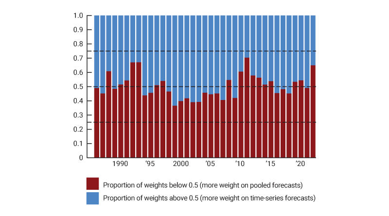
B. Noncore components
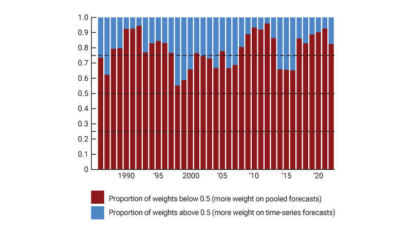
Source: Authors’ calculations based on data from the U.S. Bureau of Economic Analysis, National Income and Product Accounts of the United States, from Haver Analytics.
Figure 2 shows that noncore components (panel B) tend to place more weight on the pooled forecasts than the core components (panel A) do. This is consistent with the observation that noncore components are noisier than core components and, therefore, benefit more from borrowing strength from the panel dimension. There is less of a pattern for core components, where the split is about 50-50, indicating that for these components parameter heterogeneity and noise interact in complex ways.
Forecasting aggregate inflation
Individual weighting is a forecasting method that boosts the accuracy of forecasts for individual inflation components. That is, it improves the forecast of each inflation component by optimally exploiting the time-series and panel dimensions. But does IW also help forecast aggregate inflation? We answer this question empirically in this section.
We first aggregate the forecasts produced by each of the three methods (that is, the time-series, pooled, and IW methods) using the PCE expenditure weights of the components (see the appendix) to obtain a forecast $f_{t}^{Agg}$ for one-month-ahead aggregate PCE inflation, which we then compare with actual inflation the following month, $\unicode{x03C0} _{t+1}^{Agg}.$ We evaluate the forecasts’ accuracy using the out-of-sample R2:$5)\quad{{R}^{2}}=1-\frac{MSFE}{Var\left( \unicode{x03C0} _{t+1}^{Agg} \right)},$
which normalizes the MSFE over a particular sample by the variance of aggregate inflation over the same sample.8
Figure 3 compares the forecasting accuracy over different subperiods of aggregating the time-series, pooled, and IW forecasts of inflation components for both the AR(1) model and the intercept-only model. In both cases, we also consider as benchmarks a forecast obtained by estimating an AR(1) model on aggregate inflation directly and a forecast that uses the Cleveland Fed approach described earlier, which estimates an intercept-only model on aggregate inflation directly. We see that IW for the AR(1) model delivers the most accurate forecast for aggregate inflation (it has the largest R2) over the whole forecasting period (January 1986–December 2022) and also over the subperiods we consider. IW using the AR(1) model also outperforms IW using the intercept-only model, whereas for the other methods it is not always true that the AR(1) model dominates. These findings illustrate the importance of modeling time-varying dynamics when forecasting inflation, and also highlight the ability of IW to overcome the difficulties in estimating time-varying persistence parameters accurately.
3. Out-of-sample R2 over subperiods of the sample period
|
Jan 1986– Dec 1999 |
Jan 2000– Dec 2019 |
Jan 2020– Dec 2022 |
Jan 1986– Dec 2022 |
|
| AR(1) model | ||||
| Time-series | 0.169 | 0.009 | 0.044 | 0.115 |
| Pooled | 0.197 | 0.066 | 0.095 | 0.161 |
| IW | 0.247 | 0.083 | 0.136 | 0.188 |
| Aggregate AR(1) | 0.075 | 0.045 | –0.078 | 0.094 |
| Intercept-only model | ||||
| Time-series | 0.163 | –0.088 | 0.118 | 0.074 |
| Pooled | 0.173 | –0.149 | 0.031 | 0.027 |
| IW | 0.199 | –0.074 | 0.103 | 0.087 |
| Cleveland Fed | 0.158 | –0.096 | 0.104 | 0.066 |
Source: Authors’ calculations based on data from the U.S. Bureau of Economic Analysis, National Income and Product Accounts of the United States, from Haver Analytics.
In addition to reporting the forecasting performance over arbitrary subperiods, we can further unveil the full extent of time variation in relative performance by considering estimates of out-of-sample R2 computed over rolling windows of 12 months. These nonparametric estimates can be viewed as measures of the local (in time) forecasting performance of the different methods, and thus capture the possible time variation in out-of-sample accuracy. Figure 4 plots such a measure of the local performance for the time-series, pooled, and IW forecasts in the context of the AR(1) model (focusing on 2005 onward).
4. Out-of-sample R2 over rolling windows of 12 months for the AR(1) model
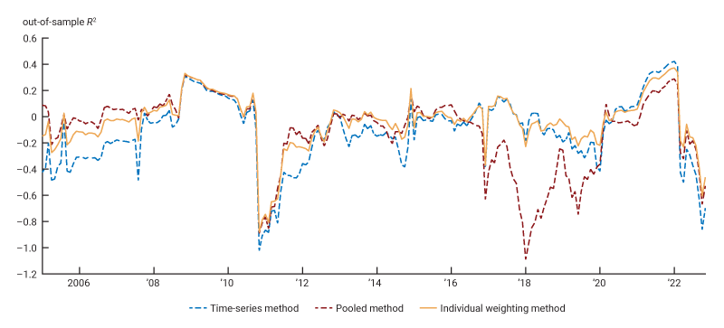
Source: Authors’ calculations based on data from the U.S. Bureau of Economic Analysis, National Income and Product Accounts of the United States, from Haver Analytics.
Figure 4 illustrates an appealing robustness property of IW. We see that the relative forecasting performances of the time-series method and the pooled method vary widely over time. Until around 2017, the pooled method generally outperforms the time-series method (a larger out-of-sample R2 in figure 4 indicates greater forecasting accuracy); however, the pooled method’s forecasting performance dramatically deteriorates in the 2017–21 period. In contrast, the IW forecasts for aggregate inflation are sometimes the best forecasts, but they are never the worst ones among the three. This robustness comes from the fact that IW flexibly lets the data decide how much strength to borrow from the panel dimension for each component and at each point in time, thus avoiding the large errors of any procedure that would always use the same forecast method for all components.9
Conclusion
In this article, we have advocated for treating inflation forecasting as a microforecasting problem. Motivated by the widespread heterogeneity in the dynamics of inflation across its components and over time, we considered a disaggregated individual weighting approach that optimally trades off the information contained in time-series and panel data. Among the forecasting approaches considered here, this method provides the most accurate forecast for aggregate inflation from the mid-1980s through 2022. This method also offers robustness properties that are highly desirable in the face of economic uncertainty and structural instability.
Notes
1 The core components of inflation exclude the more volatile food and energy components, which are the noncore components. Core inflation (based on only the inflation of the core components) is often considered by economists as a better indicator of underlying inflation trends than is total inflation (which is based on the inflation of both core and noncore components).
2 The series are not all at the same level of disaggregation because the BEA has changed the series they track over time. The 177 series currently used by the Dallas Fed (down from the original list of 186 in 2005 and the revised list of 178 in 2009) were chosen to get the finest level of disaggregation extending back to 1977. For more information, see Dolmas (2005, 2009).
3 Inflation is computed as the percent difference in prices in months t and t – 1.
4 The choice of a flat kernel gives the same weights to all points within the estimation window. One could also consider kernels with nonuniform weighting—for example, ones that give more weight to recent observations. Such weighting can be viewed as a way to capture time variation in parameters. We do not consider this alternative approach here as we want to remain agnostic about the type of time variation in the parameters.
5 The MSFE is $E\left( {{e}^{2}} \right)\text{ = }Var\left( e \right)\text{ + }{{\left[ E\left( e \right) \right]}^{2}},$ where e is the forecast error and E(e) is the forecast bias.
6 We focus on one-month-ahead forecasts, so that $f_{i,t}^{TS}={{\hat{{\unicode{x03B1 }}}_{i,t}}+{{\hat{{\unicode{x03C1 }}}_{i,t}}{\unicode{x03C0 }}}_{i,t}},$ with parameters estimated by OLS using the time series including the most recent 12 months of inflation data for component i, and $f_{i,t}^{Pool}={{\hat{\unicode{x03B1 }}}_{t}}+{{\hat{\unicode{x03C1 }}}_{t}}{\unicode{x03C0 }_{i,t}},$ with parameters estimated by pooled OLS using the panel including the most recent 12 months of inflation data for all components.
7 The first time-series and pooled forecasts for January 1985 are made using 12 months of data from January 1984 through December 1984, and the last of these forecasts for December 2022 use 12 months of data from December 2021 through November 2022. Computing the weights for IW requires 12 months of out-of-sample forecast errors for the time-series forecasts and the pooled forecasts, so the first IW forecast is for January 1986.
8 The MSFE for aggregate inflation over a sample t = 1, ..., T is computed as $\frac{\sum{_{t=1}^{T-1}{{\left( {\unicode{x03C0}} _{t+1}^{Agg}-f_{t}^{Agg} \right)}^{2}}}}{T-1}.$ Note that the out-of-sample R2 can be negative as it normalizes the MSFE by the variance of aggregate inflation over a different sample than that used for the estimation.
9 It may seem counterintuitive that the IW forecast continues to put more weight on the pooled forecast (see figure 2) even in periods where figure 4 reveals that the pooled forecasts perform poorly (for instance, during the 2017–21 period). One should, however, bear in mind that IW selects weights based on the performance of the pooled forecast for each inflation component separately, whereas figure 4 focuses on the performance of the pooled forecast for aggregate inflation. The relationship between the two is not straightforward.
Appendix: Personal Consumption Expenditures Price Index components used with our forecasting models
This appendix lists the PCE components (plus their respective expenditure weights from the BEA, averaged over our sample period of January 1984–December 2022) used with the forecasting models in this article (see figure A1). With the exception of five components (see figure A2), these components are the same ones used by the Dallas Fed to compute their trimmed mean PCE rate. (Standard clothing issued to military personnel’s expenditure weight is listed as 0.00% because of rounding.)
A1. Components used
| Component | Expenditure weight (%) |
|
| 1 | Window coverings | 0.15 |
| 2 | Spectator sports | 0.17 |
| 3 | Bicycles and accessories | 0.05 |
| 4 | Other recreational vehicles | 0.17 |
| 5 | Pleasure aircraft | 0.02 |
| 6 | Pleasure boats | 0.14 |
| 7 | Audio equipment | 0.22 |
| 8 | Eggs | 0.09 |
| 9 | Watches | 0.09 |
| 10 | Membership clubs and participant sports centers | 0.38 |
| 11 | Domestic services | 0.26 |
| 12 | Sewing items | 0.02 |
| 13 | Clothing materials | 0.06 |
| 14 | Televisions | 0.29 |
| 15 | Small electric household appliances | 0.06 |
| 16 | Other video equipment | 0.18 |
| 17 | Fruit (fresh) | 0.28 |
| 18 | Recreational books | 0.26 |
| 19 | Motor vehicle leasing | 0.36 |
| 20 | Amusement parks, campgrounds, and related recreational services | 0.44 |
| 21 | Package tours | 0.09 |
| 22 | Natural gas | 0.61 |
| 23 | Calculators, typewriters, and other information processing equipment | 0.01 |
| 24 | Telephone and related communication equipment | 0.12 |
| 25 | Outdoor equipment and supplies | 0.04 |
| 26 | Stationery and miscellaneous printed materials | 0.28 |
| 27 | Educational books | 0.11 |
| 28 | Men’s and boys’ clothing | 1.13 |
| 29 | Electricity | 1.62 |
| 30 | Vegetables (fresh) | 0.38 |
| 31 | Video discs, tapes, and permanent digital downloads | 0.14 |
| 32 | Cosmetic / perfumes / bath / nail preparations and implements | 0.44 |
| 33 | Miscellaneous household products | 0.12 |
| 34 | Other household services | 0.16 |
| 35 | Food products, not elsewhere classified | 1.19 |
| 36 | Gasoline and other motor fuel | 2.64 |
| 37 | Used light trucks | 0.56 |
| 38 | Personal computers/tablets and peripheral equipment | 0.36 |
| 39 | Cereals | 0.43 |
| 40 | Nonelectric cookware and tableware | 0.22 |
| 41 | Fuel oil | 0.23 |
| 42 | Other depository institutions and regulated investment companies | 0.91 |
| 43 | Photographic equipment | 0.06 |
| 44 | Food supplied to military | 0.02 |
| 45 | Food supplied to civilians | 0.14 |
| 46 | Higher education school lunches | 0.13 |
| 47 | Elementary and secondary school lunches | 0.08 |
| 48 | Alcohol in purchased meals | 0.71 |
| 49 | Foundations and grantmaking and giving services to households | 0.02 |
| 50 | Motor vehicle maintenance and repair | 1.59 |
| 51 | Major household appliances | 0.46 |
| 52 | Fresh milk | 0.26 |
| 53 | Games, toys, and hobbies | 0.54 |
| 54 | Prescription drugs | 2.10 |
| 55 | Household linens | 0.34 |
| 56 | Poultry | 0.45 |
| 57 | Hotels and motels | 0.67 |
| 58 | Repair of furniture, furnishings, and floor coverings | 0.02 |
| 59 | Repair of household appliances | 0.05 |
| 60 | Labor organization dues | 0.15 |
| 61 | Miscellaneous personal care services | 0.43 |
| 62 | Repair and hire of footwear | 0.01 |
| 63 | Clothing repair, rental, and alterations | 0.07 |
| 64 | New light trucks | 1.44 |
| 65 | Audio-video, photographic, and information processing equipment services | 0.99 |
| 66 | Household cleaning products | 0.42 |
| 67 | Social advocacy and civic and social organizations | 0.16 |
| 68 | Hairdressing salons and personal grooming establishments | 0.49 |
| 69 | Final consumption expenditures of nonprofit institutions serving households | 2.51 |
| 70 | Food produced and consumed on farms | 0.01 |
| 71 | Net household insurance | 0.07 |
| 72 | Elementary and secondary schools | 0.27 |
| 73 | Legal services | 0.92 |
| 74 | Professional association dues | 0.07 |
| 75 | Pari-mutuel net receipts | 0.06 |
| 76 | Casino gambling | 0.63 |
| 77 | Lotteries | 0.21 |
| 78 | Spirits | 0.24 |
| 79 | Maintenance and repair of recreational vehicles and sports equipment | 0.05 |
| 80 | Sugar and sweets | 0.46 |
| 81 | Communication | 1.92 |
| 82 | Social assistance | 0.71 |
| 83 | Standard clothing issued to military personnel | 0.00 |
| 84 | Shoes and other footwear | 0.69 |
| 85 | Nursing homes | 1.30 |
| 86 | Women’s and girls’ clothing | 1.88 |
| 87 | Processed fruits and vegetables | 0.30 |
| 88 | Water supply and sewage maintenance | 0.58 |
| 89 | Hair, dental, shaving, and miscellaneous personal care products except electrical products | 0.53 |
| 90 | Electric appliances for personal care | 0.05 |
| 91 | Proprietary and public higher education | 0.69 |
| 92 | Nonprofit private higher education services to households | 0.49 |
| 93 | New domestic autos | 0.90 |
| 94 | New foreign autos | 0.49 |
| 95 | Other purchased meals | 4.51 |
| 96 | Paramedical services | 2.21 |
| 97 | Used autos | 0.67 |
| 98 | Coffee, tea, and other beverage materials | 0.13 |
| 99 | Group housing | 0.01 |
| 100 | Tenant-occupied mobile homes | 0.09 |
| 101 | Nonprofit hospitals’ services to households | 4.55 |
| 102 | Proprietary hospitals | 0.79 |
| 103 | Government hospitals | 1.36 |
| 104 | Laundry and drycleaning services | 0.12 |
| 105 | Housing at schools | 0.19 |
| 106 | Owner-occupied mobile homes | 0.51 |
| 107 | Owner-occupied stationary homes | 10.91 |
| 108 | Rental value of farm dwellings | 0.17 |
| 109 | Flowers, seeds, and potted plants | 0.31 |
| 110 | Veterinary and other services for pets | 0.23 |
| 111 | Garbage and trash collection | 0.16 |
| 112 | Commercial banks | 1.01 |
| 113 | Religious organizations’ services to households | 0.07 |
| 114 | Computer software and accessories | 0.33 |
| 115 | Funeral and burial services | 0.23 |
| 116 | Parking fees and tolls | 0.17 |
| 117 | Dental services | 0.93 |
| 118 | Tools, hardware, and supplies | 0.21 |
| 119 | Tobacco | 0.93 |
| 120 | Carpets and other floor coverings | 0.24 |
| 121 | Beer | 0.61 |
| 122 | Other meats | 0.27 |
| 123 | Other personal business services | 0.06 |
| 124 | Physician services | 3.67 |
| 125 | Tires | 0.28 |
| 126 | Children’s and infants’ clothing | 0.18 |
| 127 | Corrective eyeglasses and contact lenses | 0.27 |
| 128 | Commercial and vocational schools | 0.33 |
| 129 | Pets and related products | 0.42 |
| 130 | Child care | 0.28 |
| 131 | Day care and nursery schools | 0.09 |
| 132 | Accessories and parts | 0.36 |
| 133 | Nonprescription drugs | 0.44 |
| 134 | Household paper products | 0.35 |
| 135 | Furniture | 1.00 |
| 136 | Bakery products | 0.77 |
| 137 | Moving, storage, and freight services | 0.16 |
| 138 | Processed dairy products | 0.41 |
| 139 | Beef and veal | 0.48 |
| 140 | Motion picture theaters | 0.11 |
| 141 | Museums and libraries | 0.06 |
| 142 | Live entertainment, excluding sports | 0.18 |
| 143 | Railway transportation | 0.01 |
| 144 | Other road transportation service | 0.10 |
| 145 | Water transportation | 0.02 |
| 146 | Intercity buses | 0.02 |
| 147 | Pension funds | 0.38 |
| 148 | Other fuels | 0.02 |
| 149 | Audio discs, tapes, vinyl, and permanent digital downloads | 0.16 |
| 150 | Financial service charges, fees, and commissions | 2.12 |
| 151 | Clocks, lamps, lighting fixtures, and other household decorative items | 0.32 |
| 152 | Intracity mass transit | 0.16 |
| 153 | Taxicabs and ride sharing services | 0.06 |
| 154 | Air transportation | 0.71 |
| 155 | Lubricants and fluids | 0.07 |
| 156 | Mineral waters, soft drinks, and vegetable juices | 0.81 |
| 157 | Luggage and similar personal items | 0.23 |
| 158 | Fish and seafood | 0.15 |
| 159 | Wine | 0.28 |
| 160 | Therapeutic medical equipment | 0.20 |
| 161 | Other medical products | 0.04 |
| 162 | Sporting equipment, supplies, guns, and ammunition | 0.55 |
| 163 | Fats and oils | 0.19 |
| 164 | Jewelry | 0.60 |
| 165 | Motor vehicle rental | 0.12 |
| 166 | Newspapers and periodicals | 0.45 |
| 167 | Pork | 0.32 |
| 168 | Film and photographic supplies | 0.05 |
| 169 | Musical instruments | 0.05 |
| 170 | Tax preparation and other related services | 0.16 |
| 171 | Dishes and flatware | 0.21 |
| 172 | Tenant-occupied stationary homes and landlord durables | 3.55 |
A2. Components excluded
| Component |
Expenditure weight (%) |
|
| 1 | Net motor vehicle and other transportation insurance | 0.61 |
| 2 | Net health insurance | 1.33 |
| 3 | Life insurance | 0.89 |
| 4 | Motorcycles | 0.10 |
| 5 | Employment agency services | 0.02 |
References
Dolmas, Jim, 2009, “The 2009 revision to the trimmed mean PCE inflation series,” Federal Reserve Bank of Dallas, technical note, August, available online.
Dolmas, Jim, 2005, “Trimmed mean PCE inflation,” Federal Reserve Bank of Dallas, working paper, No. 0506, July 25, available online.
Giacomini, Raffaella, Sokbae Lee, and Silvia Sarpietro, 2023, “A robust method for microforecasting and estimation of random effects,” Federal Reserve Bank of Chicago, working paper, No. 2023-26, August. Crossref
James, W., and Charles Stein, 1961, “Estimation with quadratic loss,” in Proceedings of the Fourth Berkeley Symposium on Mathematical Statistics and Probability, Jerzy Neyman, (ed.), Vol. 1, Contributions to the Theory of Statistics, Berkeley, CA: University of California Press, pp. 361–379, available online.
Knotek, Edward S., II, and Saeed Zaman, 2015, “Nowcasting U.S. headline and core inflation,” Federal Reserve Bank of Cleveland, working paper, No. 14-03R, revised December 2015. Crossref


