

The following publication has been lightly reedited for spelling, grammar, and style to provide better searchability and an improved reading experience. No substantive changes impacting the data, analysis, or conclusions have been made. A PDF of the originally published version is available here.
On August 22, 1996, President Clinton signed the Personal Responsibility and Work Opportunity Reconciliation Act. Among the major changes contained in the act were limits in eligibility for the Supplemental Security Income and Food Stamp programs and an end to the entitlement of families with children to cash assistance. The act replaced the cash assistance program, Aid to Families with Dependent Children (AFDC), with Temporary Assistance to Needy Families (TANF). The AFDC program had been an open-ended matching grant program, where federal grants grew in line with state expenditure. By contrast, the TANF program is a fixed block grant. While a block grant gives states greater flexibility, more financial independence, and the ability to innovate, it also renders the federal grant amount to a state independent of the state’s changing needs over the business cycle. In this Chicago Fed Letter, I compare the relationship between federal and state welfare spending and state budgets under the AFDC program and under the first two years of the TANF program.
State budgets under AFDC
Under AFDC, all eligible families in a state received a monthly benefit that was set by the state. The federal government paid for half of the program’s administrative costs and a portion of the state’s benefit payments, which was tied to the state’s per capita income.
Under the matching grant system, the money coming from the federal government increased during times of economic hardship in the state. If the state economy worsened and caseloads swelled, the state and federal governments shared the increased costs. Therefore, federal grants were countercyclical in nature. Figure 1 illustrates the relationship between state government budgets, public welfare spending, federal intergovernment welfare transfers, and the business cycle from 1988 through 1996.
1. State budget items and the business cycle, 1988–96
| Effect of 1 percentage point increase in fiscal year unemployment | T-statistic | |
| (1997 $ per capita) | ||
| Total revenue | 2.08 | 0.21 |
| Total expenditure | 52.04 | 6.92 |
| Cash assistance spending | 8.55 | 9.77 |
| All public welfare spending | 29.76 | 10.22 |
| Federal intergovernment grants for public welfare received by state | 13.68 | 5.88 |
| Income tax revenue | -10.30 | 2.71 |
Source: Author’s tabulations using state finance data from U.S. Department of Commerce, Bureau of the Census, 1998, State Government Finances, and unemployment rate data from the U.S. Department of Labor, Bureau of Labor Statistics, 1998, “Local area unemployment.”
The figure demonstrates the importance of federal government public welfare grants in mitigating the effects of the business cycle on state budgets. The first row of the figure shows that total state revenue is practically independent of the business cycle. By contrast, the second row demonstrates that state expenditure is very responsive to the business cycle—a 1 percentage point increase in the state’s fiscal year unemployment rate (e.g., a jump from 6% to 7%) increased state per capita expenditure by $52.
The data presented in the third and fourth rows of figure 1 show that approximately 15% of this increase was driven by increases in cash assistance spending ($8.55 of $52.04), while more than half of the increase was driven by increases in overall public welfare spending ($29.76 of $52.04). Cash assistance spending is defined as direct cash payments to needy recipients. Public welfare spending includes cash assistance spending, vendor payments for medical care and other purposes, and spending for other welfare programs. From these two rows it is clear that during times of high unemployment, states expended more resources assisting the needy.
Figure 1 also shows that between 1988 and 1996 at the same time that state government public welfare spending increased, public welfare grants from the federal government increased. Row five shows that about half the increase in public welfare spending was financed by grants from the federal government.
The final row of figure 1 depicts the decline in state income tax revenues that occurs when the state economy worsens. A comparison between the coefficients in rows five and six reveals that the growth in federal government welfare grants approximately compensated for the decline in income tax revenues brought about by a declining economy.
The switch to TANF
The provisions of the Personal Responsibility and Work Opportunity Reconciliation Act give states a fixed nominal block grant to spend on the programs replaced with TANF for each fiscal year from 1997 through 2002. In addition to replacing AFDC, the TANF block grant is also to be used to fund programs previously supported by the much smaller Job Opportunity and Basic Skills and Emergency Assistance funds. The amount of the block grant is the maximum of the federal contribution to these programs in federal fiscal year 1994, in federal fiscal year 1995, or the average of the federal contribution between federal fiscal years 1992 and 1994.
The total amount of the block grants for 1997–2002 is $16.4 billion per year, which represents a 9% increase over total federal TANF-related program spending in 1996.1 Figure 2 shows that the original federal endowments were generous in general and very generous for the Seventh District states overall.
2. Federal welfare grants to Seventh District states
| Programs replaced by TANF, 1996 | TANF block grant 1997-2002 | Percent change | |
| (millions of nominal dollars) | |||
| Illinois | 593 | 585 | -1 |
| Indiana | 121 | 207 | 70 |
| Iowa | 124 | 132 | 6 |
| Michigan | 581 | 775 | 33 |
| Wisconsin | 240 | 318 | 33 |
| Seventh District | 1,660 | 2,017 | 22 |
| U.S. | 14,992 | 16,396 | 9 |
In addition to federal funds, the law contains a maintenance of effort (MOE) provision that requires states to continue to spend 75% of the money they had spent in fiscal year 1994 out of their own budgets on the programs replaced by TANF. While the federal block grant money must be spent on families that meet certain work requirements and time limits, states have a great deal of freedom as to how they spend their MOE funds.
In recognition of the fact that states usually need more resources in difficult economic times, the law provides two additional sources of funds in the event of a recession—a $2 billion contingency fund and a $1.7 billion rainy day loan fund. The contingency fund allows a state to receive a maximum of 20% of its yearly block grant in any year in which it has a sufficiently high unemployment rate or sufficiently high growth in its food stamp population. The loan fund allows a state to borrow up to 10% of its grant for up to three years. In addition, although states are required to spend their MOE funds in a given fiscal year, they do not need to spend their entire block grant. States are permitted to leave some of the block grant for future use on account at the U.S. Treasury.
The states had until July 1, 1997, to put into effect a plan to achieve the goals of the TANF program. However, states could switch to TANF earlier if their plan for using the funds was accepted. Because of the healthy state of the economy following the law’s passage, the matching grant levels were lower than the block grant levels and states had an incentive to switch to TANF as early as possible.
The first years of TANF
In the two plus years since the enactment of the TANF program, the new law has been a windfall to state government budgets. The strength of the economy contributed to a 35% decline in recipient families between January 1996 and June 1998.2 Under AFDC, the decline in caseloads would have led to a drop in the grants coming from the federal government. Under TANF, the grants remained at their legislated levels. In addition, the low inflation rate during this period meant that the real value of the fixed nominal grant was only minimally eroded.
The decline in caseloads combined with the increase in federal government spending has meant that states have been able to spend more money on each recipient. The Government Accounting Office (GAO) estimated the difference between the minimum level of funds available under TANF (the sum of MOE and the block grants) and the amount that the states and federal government would have spent on their 1997 caseloads if they were still operating under the AFDC cost structure. It found that states had an additional $4.7 billion to spend under TANF than they would have had under AFDC.3
States have used these additional funds in a variety of ways. In general, states have increased their spending on support services. State and federal childcare expenditures for 1998 are expected to be 69% higher than in 1996, and expenditures on job training and placement programs are estimated to be 58% higher in 1998 than they were in 1996.4 In addition, some states have not spent these additional resources, but have left them on account at the Treasury. According to the GAO, as of September 30, 1997, states had $1.2 billion in unspent balances remaining at the U.S. Treasury. The GAO points out that it is unclear whether these unspent funds were the result of deliberate contingency planning by the states or an outgrowth of the transitional nature of TANF during its first year. Importantly, states are limited in their ability to develop their own dedicated welfare reserve funds, because money deposited in a reserve fund does not count toward the state MOE requirement in the year it was deposited.
TANF during a recession
While welfare reform has been a windfall for the states in this period of economic expansion, the opposite would be true during a time of economic decline. Were unemployment rates to increase, caseloads would likely grow and demands on state budgets would likewise increase. At the same time, the TANF block grant would remain at its specified nominal level.
How states will deal with these increased demands is an open question. Because most states operate under balanced budget requirements and debt limits, they will for the most part be unable to finance heightened welfare spending by borrowing against future resources. States will essentially face five choices. They could increase or maintain their total welfare spending by decreasing spending in other areas or by increasing taxes. They could decrease welfare spending by cutting programs and benefit levels or by restricting eligibility. They could spend money saved in rainy day funds or money maintained at the Treasury. They could access loan or contingency funds. Finally, they could lobby Congress to change the law and increase the level of spending.
At the beginning of a downturn, states may well be able to fund increased welfare spending using money saved in rainy day funds or at the Treasury or by decreasing spending in other areas. In the late 1990s nearly all states have shown impressive budget surpluses. States have both returned money to their citizens and beefed up balances. Figure 3 depicts year-end balances as a percent of spending in fiscal 1998 in the U.S. as a whole and in the Seventh District. The magnitude of these balances suggests that states may be able to maintain service levels for a while following an increase in their welfare rolls by drawing down balances.
3. 1998 year-end balances
| Percent of expenditure | |
| Illinois | 3.9 |
| Indiana | 20.5 |
| Iowa | 18.7 |
| Michigan | 12.1 |
| Wisconsin | 3.7 |
| United States | 6.0 |
Source: National Association of State Budget Officers, 1998, Fiscal Survey of the States, May.
However, if a downturn proves lengthy, these balances may dry up. In that case, one option would be for states to maintain benefit levels by increasing taxes. However, given the contentious nature of legislation for tax increases, it is unlikely that they would be enacted in a timely manner. It is also unlikely that states would use the contingency or rainy day loan fund provisions in the TANF legislation. Use of the contingency fund requires states to spend 100% of their fiscal 1994 expenditures for a limited set of purposes. This requirement, combined with the need to meet the unemployment or food stamp triggers, renders the contingency fund a complex source of funds. Even if states do choose to access the contingency funds, the funds are not large enough to help many states for more than a short period. The rainy day loan fund is not very attractive to states either. State officials reported to the GAO that borrowing for increased welfare spending is unlikely to be politically popular during a recession.5
This leaves states with two choices. They can cut benefits or they can turn to the federal government for help. After drawing down balances, states will probably need to cut welfare spending. This is unfortunate because it would result in an interruption of services at the time when such services were most needed. Moreover, in order to receive their full government grant, states need a portion of their caseload to meet certain work requirements. During a period of high unemployment, finding or creating work for recipients will be both difficult and costly. With more money going toward work requirements, benefit levels would need to shrink. A decline in benefit levels would most likely lead both state officials and advocacy groups to pressure the federal government to appropriate more funds for the program.
Over time, other reasons to change the law will probably surface. For example, fixed nominal block grants based on mid-1990s spending levels will ultimately become outdated. Ideally, changes in the law would explicitly take into account the relationship between public welfare demands and the condition of the labor market by making the level of block grants and the nature of work requirements dependent on the state economy.
Conclusion
In this Chicago Fed Letter, I have explored the relationship between the business cycle and state and federal public welfare spending before and after welfare reform. While prior to welfare reform, federal government transfers were countercyclical, the passage of the Personal Responsibility and Work Opportunity Reconciliation Act made federal cash assistance grants independent of the business cycle. This change has been a windfall for state budgets in the period immediately following welfare reform because of the health of the economy. However, state budgets would be subject to increased fiscal pressures in the event of a downturn. While the size of recent budget surpluses suggests that most states would be able to cope with a brief downturn, a prolonged recession could lead to disruptions in state welfare programs and, ultimately, to changes in the TANF program.
Tracking Midwest manufacturing activity
Manufacturing output indexes (1992=100)
| September | Month ago | Year ago | |
|---|---|---|---|
| CFMMI | 124.8 | 125.9 | 122.1 |
| IP | 131.3 | 131.9 | 128.0 |
Motor vehicle production (millions, seasonally adj. annual rate)
| October | Month ago | Year ago | |
|---|---|---|---|
| Cars | 6.1 | 6.5 | 5.9 |
| Light trucks | 6.6 | 5.9 | 6.2 |
Purchasing managers' surveys: net % reporting production growth
| October | Month ago | Year ago | |
|---|---|---|---|
| MW | 57.3 | 67.8 | 62.6 |
| U.S. | 52.6 | 53.4 | 59.6 |
Manufacturing output indexes, 1992=100
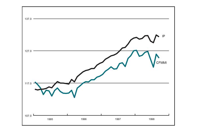
The Chicago Fed Midwest Manufacturing Index (CFMMI) decreased 0.9% in September following a revised 3.3% gain in August. The Federal Reserve Board’s Industrial Production Index for manufacturing (IP) fell 0.4% in September following an increase of 1.8% in August. Car production decreased to 6.1 million units from 6.5 million units. Light truck production increased to 6.6 million units in October from 5.9 million units in September.
The Midwest purchasing managers’ composite index (a weighted average of the Chicago, Detroit, and Milwaukee surveys) for production decreased to 57.3% in October from 67.8% in September. Purchasing managers’ indexes decreased in Chicago, Detroit, and Milwaukee. The national purchasing managers’ survey for production declined from 53.4% to 52.6% from September to October.
Notes
1 U.S. General Accounting Office, 1998, Welfare Reform: Early Fiscal Effects of the TANF Block Grant, letter report, No. GAO / AIMD-98-137, August 18.
2 U.S. Department of Health and Human Services, The Administration for Children and Families, “Changes in welfare caseloads as of June 1998,” available at www.acf.d hhs.gov.
3 U.S. General Accounting Office, 1998, op. cit.
4 Data from National Association of State Budget Officers, 1998, Special Feature: Welfare Reform. The percent changes are in nominal dollars because the 1998 GDP deflator is not yet available. The childcare number omits six states and the work program number omits five states due to unavailability of data.
5 U.S. General Accounting Office, 1998, op. cit.


