Life insurers sell protection against adverse life events. They receive payments from policyholders during good times, and they pay policyholders when something goes wrong. They also sell savings instruments, usually associated with a guaranteed (minimum) return that protects policyholders from market downturns. For both products, life insurers receive payments from policyholders early on and make payments to them later. In the meantime, insurers buy financial assets such as bonds, real estate, or stocks that in general they hold until they must make payments to policyholders.
This business model exposes insurers to at least these two sources of risk: credit risk, which is the risk that the financial assets’ default probability increases, reducing their value below the value of the obligations with policyholders; and interest rate risk, which is the risk that a change in interest rates (that in turn changes the discount rate) increases the net present value of obligations with policyholders relative to the net present value of the assets. In this Chicago Fed Letter, I study interest rate risk.1
Insurers’ exposure to interest rate risk arises because interest rate changes might affect liabilities and assets differently. However, if the cash flows of the assets and the cash flows of the liabilities were identical, any change in the value of the liabilities due to a change in interest rate would be offset by an equally large change in the value of the assets. Hence, insurers can reduce this risk exposure by matching assets and liabilities’ cash flows. Because matching cash flows is operationally complex, insurers usually match duration, which is a measure of how the cash flows are distributed over time. When cash flows are received or paid far in the future, the duration is long, whereas when cash flows are paid or received in the short term, the duration is short.
When the duration of liabilities is closely matched with the duration of assets, the exposure to interest rate risk is small. The opposite is true when the matching is poor. In the case of insurers, observing the degree of duration-matching is challenging because information on liability maturity is not publicly available. However, I can measure the matching indirectly by studying how the value of insurers’ equity is affected by changes in interest rates. As I stated before, if the duration-matching is effective, then changes in the value of liabilities due to changes in interest rates would be largely offset by a similar change in the value of the assets and hence, would have a minimal effect on the value of equity. The degree to which equity value changes when interest rate changes is usually referred to as interest rate sensitivity.
In a world where interest rates were the only variable affecting the value of assets and liabilities, measuring the interest rate sensitivity would be straightforward. I would measure the change in the value of life insurers’ equity for a given change in the interest rate and take the ratio of these changes. In real life, however, there are multiple variables affecting the value of assets and liabilities. For example, unemployment, gross domestic product (GDP), and mortgage delinquency, among many others, might have a significant effect on assets and liabilities, making the measuring of sensitivity more challenging. Omitting these variables could strongly bias the estimation. In this article, I propose a new approach to estimating the sensitivity of life insurers that addresses the challenges associated with measuring interest rate sensitivity when omitted variables are relevant. The idea underlying this approach is simple: If I can find a window of time when changes in interest rates are large relative to changes in other economic variables, I could reduce the distortions associated with other variables by narrowing down the estimation to this window of time.
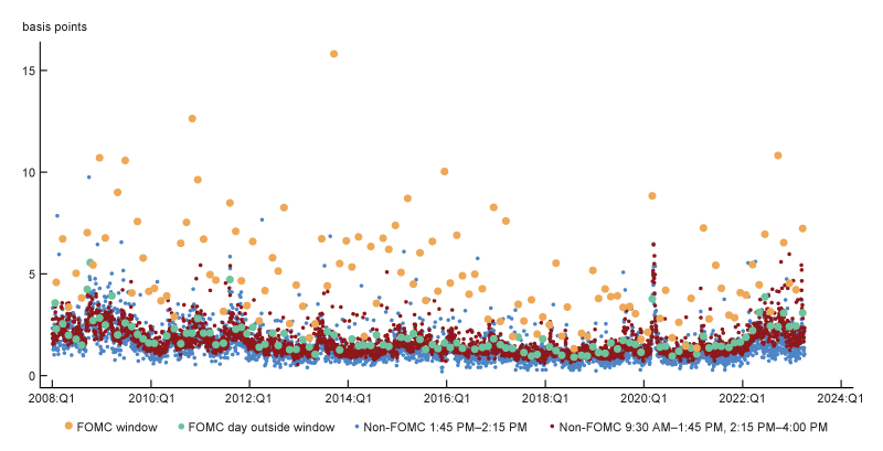
It turns out such time windows do exist. In figure A3 of the appendix, I can observe that the standard deviation of the returns on a ten-year Treasury bond, which I use as the measure of changes in interest rates, is an order of magnitude larger during a narrow window before and after a fed funds rate announcement by the Federal Reserve’s monetary policymaking body, the Federal Open Market Committee (FOMC). Given the large magnitude of interest rate changes, it is likely these changes dominate changes in other variables during these windows, making the measure of sensitivity more accurate. I run an ordinary least squares (OLS) estimation to find the ratio of changes in equity value to changes in interest rates that best fits the data. To further reduce the concerns that other variables might distort our estimation, even during the narrow FOMC windows, in the OLS estimation I add a control for the return on a broad stock market index.
I am not the first to introduce FOMC window analysis to improve the estimation of interest rate sensitivities. This idea has already been used for banks (see, e.g., Kuttner (2001), Gürkaynak, Sack, and Swanson (2005), and English, Van den Heuvel, and Zakrajšek (2018)). However, they use the overall change in interest rate and the overall change in equity prices on each FOMC announcement day as a single data point and estimate a time-series regression over a long horizon. Instead, using high-frequency pricing data, I estimate the sensitivity of returns at the minute level during the period from 15 minutes before each FOMC announcement to 15 minutes after the announcement.
In my estimation, the change in life insurers’ equity value, measured as the return on a broad life insurance index, is the left-hand side variable, and the changes in the interest rate, measured as the returns on a ten-year Treasury bond, is the explanatory variable. I also add the return on a broad stock market index (the S&P 500) as an explanatory variable to control for changes in life insurers’ equity value due to stock market fluctuations. Because the time windows are short, I need high frequency pricing (one-minute returns) to run my model.
My results using short time windows around FOMC announcements suggest that an increase in interest rates is neutral to life insurers’ equity prices before 2016 and increases the value of life insurers’ equity after that. To benchmark my results with previous work, I also estimate the sensitivity using all times on all trading days. In my calculations, the sensitivity estimated around FOMC announcements is significantly different from the sensitivity estimated using all dates. The differences are largest during the 2007–08 global financial crisis and during the 2015–19 Fed monetary policy tightening. These results suggest there could be a strong bias in the interest rate sensitivity estimation when measured during days or times of day when the variation of interest rates could be mudded by the variation of other relevant economic variables.
Methodology
I use ordinary least squares to estimate the return on life insurers’ equity index as a function of the return on a ten-year Treasury bond, which I use as my measure of the interest rate. While the maturity of life insurers’ assets and liabilities is longer than ten years, the ten-year Treasury is traded more often, making high-frequency prices more representative relative to longer horizon bonds that trade more sporadically. In the regression, I also control for the return on a broad stock market index—to reduce concerns of omitted variables that also affect the broad economy.
Specifically, I follow Hartley, Paulson, and Rosen (2016) in estimating the following regression:
1) rit = α + βrmt + γryt + ϵit ,
where rit is the return on the life insurance index on date t, rmt is the return on the broad market index on date t, and ryt is the return on the ten-year Treasury on date t. However, to take advantage of the additional information embedded in more-frequently measured returns, I change the timing of the regression from daily to minute level. This change results in the following specification:
2) rijt = αt + βtrmjt + γtryjt + ϵijt ,
where { αt , βt , γt } are day-specific coefficients for the constant, the sensitivity to the broad stock market, and the sensitivity to the ten-year Treasury, respectively. Here, r is the abbreviation of returns, subscript i represents the industry, which in this case is life insurers only, subscript j captures the one-minute period within day t, m represents the market estimated as the S&P 500 stock index, and y represents the ten-year Treasury used to capture variation in interest rates. By estimating daily sensitivities with minute-level data, I can observe how the sensitivity evolves over time.
In my main estimation, I restrict the time to a window that spans from 15 minutes before to 15 minutes after an FOMC announcement, i.e., 30 observations on each (daily) regression. Then I estimate daily coefficients, αt , βt , γt . To benchmark my results with earlier methodologies, I also estimate the regression in each day on all trading times. My data sample spans the period from 2008 through 2022. I use 124 FOMC announcements within this time frame. I use robust Huber–White standard errors.
Results
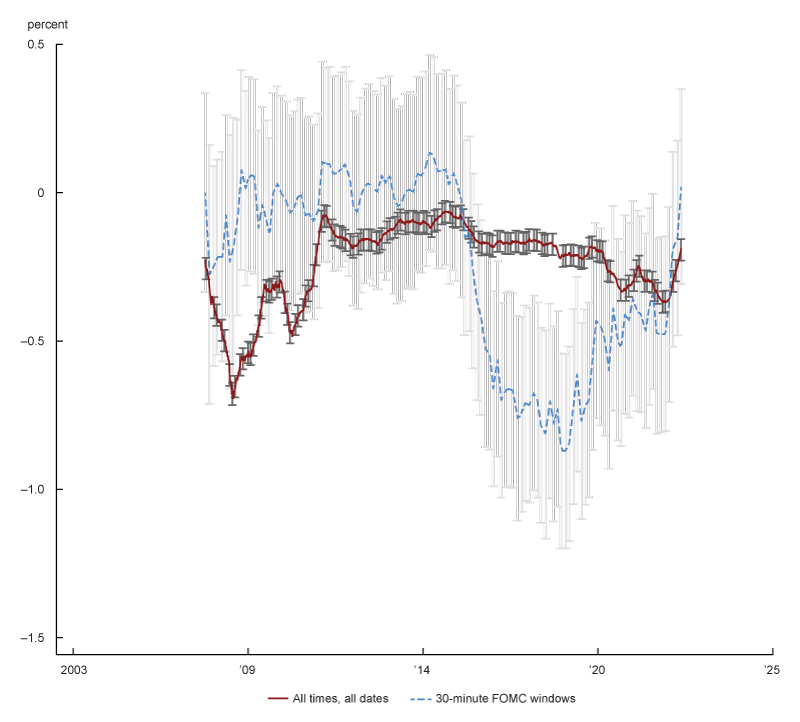
In figure 1, I present my findings. The light gray dashed line shows the sensitivity of life insurers’ market equity returns to the ten-year Treasury returns measured over a 30-minute window around a single FOMC announcement. To smooth out outliers, I plot the (rolling) average of the estimation over a period of 12 months (i.e., eight estimations, as the FOMC meets eight times a year). The black line displays the sensitivity measured in all business days and at all trading hours. I estimate the model independently for each day, and I plot the average sensitivity over a period of 12 months. Although when measuring the sensitivity every day, 12 months comprise about 250 estimations.2
1. Life insurers’ equity sensitivity to interest rate

Source: Author’s calculations using intraday pricing data.
The first thing one notices in the chart are the striking differences between the estimation around FOMC announcements and the estimation using all dates and during all times. This highlights that measuring sensitivity during periods of high variation in interest rates, such as the times around FOMC announcements, is recommended to get an unbiased measure of sensitivity. Second, the sensitivity using a narrow window around FOMC announcements is of equal or larger magnitude than the sensitivity using all dates at all times (except during the financial crisis when the interpretation of the measure is challenging). This might be a consequence of a downward bias of the sensitivity measured at all times (see Hausman, 2001). My reasoning is that measuring sensitivity to interest rates when other (excluded) variables are relevant is equivalent to using a noisy measure of the interest rate.
Using the unbiased measure of interest rate sensitivity, I observe that before 2015, changes in the interest rate did not affect life insurers’ equity value. After 2015, a decrease in the value of the Treasury bond that is equivalent to an increase in interest rates increases the value of life insurers’ equity. This is consistent with life insurers’ liabilities being of longer maturity relative to their assets, and therefore decreasing more than assets (i.e., a net benefit for life insurers’ equity value) when the interest rate increases.
Conclusion
I estimate the sensitivity of life insurers’ market equity valuation to changes in interest rates. I conduct my analysis using short time intervals around FOMC announcements to reduce potential bias associated with measurement noise and with concurrent changes in other economic factors. I find that an increase in interest rates increases life insurers’ market equity valuation, and the increase is significant both economically and statistically. This suggests previous work using all-day pricing might be subject to downward bias.
Notes
1 Insurers are also exposed to mortality risk and liquidity risk. Mortality risk is the risk that mortality increases suddenly and consequently life insurance claims increase quickly as well. Liquidity risk is associated with policyholders or other liability holders withdrawing their claims earlier than anticipated, generating cash needs beyond what the insurer can meet.
2 The standard deviation of the estimators on each day are calculated using the methodology in White (1980). The standard deviation of the eight-day rolling average is estimated assuming the standard errors on each daily estimation are independent.
Appendix
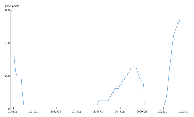
A1. Fed funds rate

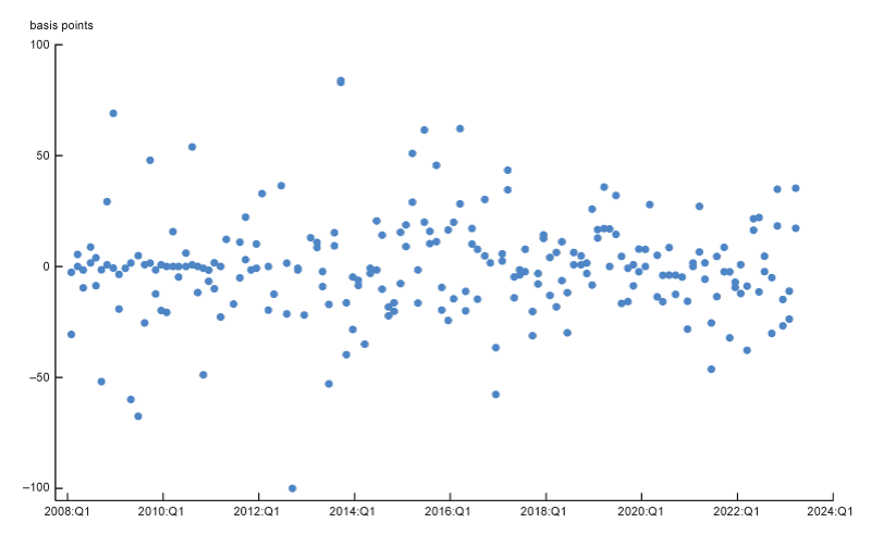
A2. Interest rate shock: Returns 15 minutes before and after FOMC announcements (30-minute window)

A3. Ten-year Treasury bond one-minute returns’ standard deviations


