

Introduction and summary
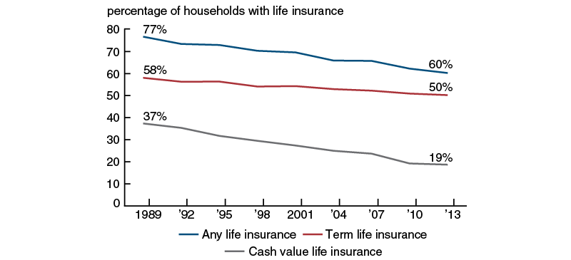
Life insurance ownership has declined markedly over the past 30 years, continuing a trend that began as early as 1960. In 1989, 77 percent of households owned life insurance (see figure 1). By 2013, that share had fallen to 60 percent. This article analyzes factors that might have contributed to the decline in life insurance ownership from 1989 to 2013. The focus of our analysis is on two broad sources of potential change in the demand for life insurance: changes in the socioeconomic and demographic characteristics of the population and changes in how those same characteristics are associated with the decision to purchase life insurance. In addition, we highlight the considerable diversity in life insurance ownership across education, income, and race and ethnicity and describe how trends in life insurance ownership vary across these groups.
Life insurance protects families from adverse financial consequences when a policyholder dies. In addition, some life insurance policies facilitate tax-advantaged savings. According to a 2015 LIMRA survey (see table 1), the top three reasons for purchasing life insurance are to cover funeral expenses (51 percent), to replace lost income (34 percent), and to cover mortgage debt (26 percent). Transferring wealth to the next generation is a close fourth, with 24 percent of respondents reporting that this was a major reason for purchasing life insurance.
We analyze 1989 and 2013 Survey of Consumer Finances (SCF) data and find substantial differences in the propensity to own life insurance among households with different demographic and socioeconomic characteristics. One fact that stands out is the high life insurance ownership rates of African American households. African American households are more likely to own life insurance than otherwise similar white households. This is in stark contrast to African American ownership of other financial assets, suggesting that there is something special about life insurance. We speculate that one factor may be the important role of African American-owned life insurance firms from the early 1920s through the 1960s (Heen, 2009; and Chapin, 2012). Another possible explanation is that higher mortality rates for African Americans make it optimal for more African Americans than whites to choose to own life insurance. However, there is evidence that African Americans, on average, expect to live six years longer than their actuarial life expectancy while whites’ subjective and actuarial life expectancies are much closer (Mirowsky, 1999). Deepening our understanding of the high rates of life insurance ownership among African Americans is an important topic for future research.
Table 1. Reasons for purchasing life insurance
|
|
Major reason |
Minor reason |
|
|
( - - - - - - - - - percent - - - - - - - - - ) |
|
|
To cover burial and final expenses |
51 |
33 |
|
To replace lost income |
34 |
24 |
|
To pay off mortgage |
26 |
17 |
|
To transfer wealth to next generation |
24 |
34 |
|
To pay for home care |
17 |
20 |
|
To supplement retirement income |
14 |
28 |
|
To pay for estate taxes or create estate liquidity |
14 |
27 |
|
As tax-advantaged way to save and invest |
8 |
23 |
|
Parent or relative bought for me |
8 |
8 |
|
To provide funds for education |
9 |
14 |
|
For business purposes |
5 |
10 |
|
To make a charitable gift |
4 |
11 |
We show that the substantial decline in life insurance ownership, driven by a steep drop in cash value policies and a more moderate drop in term policies from 1989 to 2013, is somewhat surprising given trends in socioeconomic and demographic factors. If people in 2013 behaved the same way they did in 1989, life insurance ownership would have increased modestly. Instead, ownership has decreased substantially across a wide swath of the population. Explanations for the decline in life insurance must lie in factors that influence many households rather than just a few. This means we need to look beyond the socioeconomic and demographic factors that are the focus of our analysis. A decrease in the need for life insurance due to increased life expectancy is likely to be an especially important part of the explanation. In addition, other potential factors include changes in the tax code that make the ability to lower taxes through life insurance less attractive, lower interest rates that also reduce incentives to shelter investment gains from taxes, and increases in the availability and decreases in the cost of substitutes for the investment component of cash value life insurance.
The rest of the article is organized as follows. The next section provides a brief review of related literature. Then we describe the data that we use in the analysis, along with broad trends in life insurance ownership by education, income, and race. We then investigate the characteristics associated with the demand for life insurance and consider whether changes in those factors explain the decline in life insurance ownership.
Related literature
There is an extensive theoretical and empirical literature that analyzes the demand for life insurance. Our starting point is the model developed in Lewis (1989), which extends earlier work by Yaari (1965). Lewis models the demand for life insurance by considering the perspective of potential beneficiaries and their needs in the case of the death of the insured, who is assumed to be the primary wage earner. Fischer (1973) also emphasizes the role of life expectancy in determining the demand for life insurance over the life cycle in a model where agents make decisions about savings, consumption, and insurance. Informally, in the framework from Lewis, with actuarially fair prices, the primary wage earner’s life will be insured at a level that ensures that children and a surviving spouse do not suffer financially if the primary wage earner dies prematurely. More formally, the demand for life insurance at any given point in time can be expressed as: $$1)\left( 1-lp \right)F=\underset{{}}{\mathop{\max }}\,\left\{ {{\left[ \frac{1-lp}{l\left( 1-p \right)} \right]}^{{}^{1}/{}_{\delta }}}TC-W,\text{ }\!\!~\!\!\text{ }0 \right\},\text{ }\!\!~\!\!\text{ }$$ where F is the face value of all insurance written on the primary wage earner’s life, l is the cost of the insurance divided by its actuarial value,1 p is the probability that the primary wage earner dies, $\delta $ is a measure of relative risk aversion, TC is the present value of the consumption of each child and the surviving spouse from the current period until the age at which they are assumed to live independently, given their projected life span, in the scenario that the primary wage earner does not die, and W is net household wealth.
Demand for life insurance, the left-hand side of the equation, is expressed as the face value of life insurance minus the expected premiums, in present value terms. The right-hand side of the equation reflects the primary motivation to purchase insurance: to provide consumption for states of the world in which wealth is insufficient to maintain the desired (or optimal) level of consumption. Thus, the purchasing decision comes down to comparing the adjusted present value of the consumption of the dependents (TC ) to net household wealth (W ), where the adjustment term depends on the probability that the breadwinner dies, the price of the insurance, and the risk aversion of the dependents.2
This framework provides some guidance about the factors that might influence the demand for life insurance. In particular, the demand for life insurance will be higher when the probability of death is higher, when risk aversion is higher, and when the present value of beneficiaries’ consumption is higher. The present value of beneficiaries’ consumption summarizes many factors and is likely to be higher when household income is higher, when children are younger, when the expected educational costs of children are higher, when there are more children, and when there is a single wage earner in the family. In contrast, the demand for insurance will be lower when wealth is higher and when insurance is more expensive relative to its actuarially fair value.
While the Lewis framework is useful for considering which factors may influence demand from a purely insurance perspective, other considerations may also be important. For example, tax policy is likely to influence the demand for life insurance. First, in general, the proceeds from life insurance policies paid to the beneficiaries upon the death of the insured are not taxed as income to the beneficiary and in certain situations may not be subject to the estate tax either.3 Second, life insurance policies with a savings component, sometimes referred to as “cash value” insurance products, are not subject to capital gains taxes on any growth of the initial investment. This feature is similar to that of certain retirement and educational savings plans such as Roth IRAs and 529 college savings plans.
In addition to tax considerations, households may be motivated by a desire to leave bequests to future generations. Bernheim (1991) analyzes the demand for life insurance in the context of ascertaining the degree to which household savings are driven by a bequest or purely precautionary (or insurance) motive. His idea is that Social Security endows households with an annuity and that households who wish to transfer that annuity to their children will purchase life insurance, which can be thought of as selling an annuity. He estimates life insurance demand as a function of Social Security benefits, lifetime resources (the actuarial value of private pension and Social Security benefits plus accumulated net lifetime earnings), the presence of children, widowed or widower status, marital status, and age. He finds that the propensity to hold life insurance and the amount of life insurance held are positively related to Social Security benefits, lifetime resources, and the presence of children. They are negatively related to age and widowed or widower status. His estimates are based on an analysis of the 1975 wave of Longitudinal Retirement History Survey respondents who were 64 to 69 years old.
Consistent with the theoretical literature that emphasizes the role of life insurance in protecting survivors when a primary breadwinner dies, Liebenberg, Carson, and Dumm (2012) identify a significant positive relationship between important life events, such as marriage or the birth of a child, and the demand for life insurance. Their study also finds support for the “emergency fund” hypothesis, where households that are hit by an unemployment shock are more inclined than others to use cash value life insurance to smooth shocks by surrendering cash value life insurance policies to provide extra income during the period of unemployment.
Chen, Wong, and Lee (2001) study changes in the demand for life insurance from 1949 to 1996 in the United States. They note that the decrease in the purchase of life insurance is especially prominent among households whose members belong to more recent birth cohorts. Their analysis attributes the decline in life insurance ownership over this period to two main factors: a higher share of individuals living alone without dependents and trends toward getting married later in life, which often delays the decision to have children. Brown and Goolsbee (2002) document a drop in the price of term life insurance in the late 1990s, coinciding with the introduction of internet sites that allowed for easy comparison of insurance costs. This development is likely to have reduced search costs for shopping for term life policies. In contrast, the prices of insurance products, such as whole life, not covered by the comparison sites (due to higher product heterogeneity) were not affected.
Mulholland, Finke, and Huston (2016) study the role of demographic and tax code changes that occurred from 1992 through 2010 in the decline in ownership of cash value life insurance. They found some evidence in line with the hypothesis that there was less demand for cash value life insurance in the wake of the 1998 introduction of saving vehicles, like the Roth IRA, with tax advantages similar to those of life insurance, allowing investments to grow in value tax free, for example. They were unable to find evidence that changes in estate taxation levels have influenced life insurance demand, however. This may be due to a lack of power in their test, given the small number of households for whom changes in the estate tax are consequential.
Our data
We use data from the Survey of Consumer Finances (SCF) to analyze trends in life insurance ownership. The SCF is administered by the Board of Governors of the Federal Reserve System every three years and provides comprehensive financial and demographic data for U.S. households. We analyze the earliest and latest waves of the SCF with consistent questions and methodologies, 1989 and 2013, and restrict our attention to households whose heads are between the ages of 18 and 75.1 Following the literature that emphasizes the importance of household characteristics in the decision to purchase life insurance, we study life insurance ownership at the level of the household.
There are two technical factors that are important to address in using the SCF data: weighting and imputation. Each SCF data set contains weights that indicate the number of households in the population that are represented by each household in the sample. We apply these weights to the data, which corrects for the over-sampling of wealthy households and makes the analysis representative of U.S. households. In addition, the SCF uses a multiple imputation process to estimate a value for questions that the respondent did not answer. This process creates five observations or “implicates” for each survey respondent. For our analysis, we select one of the five implicates at random.
The SCF asks respondents if they own any life insurance and specifically whether they own “term” insurance or “cash value” insurance.5 Term life insurance pays out if the policyholder dies during the term of the policy, the specified period that the policy is in force. Once the term is over, there is no payout should the policyholder die. In purchasing a term policy, a household has to decide how long they want coverage for (the term) and how much coverage they want (the payout in the event of a death during the term). Term life insurance has no savings element and is an important tool for households who desire coverage for a specific period: to provide funds for raising children if a parent dies prematurely, for example. Term policies are usually offered for periods ranging from five to 30 years and premiums depend on factors such as the policyholder’s age, health, and life expectancy. Cash value policies are sometimes called “whole life,” “straight life,” or “universal life” policies. As with term policies, cash value policies pay out if the policyholder dies. However, cash value policies differ from term policies in two important respects. First, cash value life insurance typically provides coverage for the entirety of the policyholder’s life, rather than for a specific number of years. Second, cash value life insurance allows policyholders to amass value over time. Policyholders choose how their premiums will be invested and investment earnings are credited to their accounts. Interest and investment returns on the savings components of a cash value life insurance policy accumulate tax free and there is effectively no government-imposed contribution limit to cash value life insurance policies. These features can make cash value policies an attractive tax shelter, particularly for wealthier households.
Figure 1. Life insurance ownership
Source: Authors’ calculations based on data from the Board of Governors of the Federal Reserve System, Survey of Consumer Finances.
Understanding the decline in life insurance ownership
Life insurance ownership has declined in every SCF survey year since 1989. These trends are summarized in figure 1 and table 2. Overall life insurance ownership fell by 16.5 percentage points from 1989 to 2013, going from 76.7 percent to 60.2 percent, a 21.5 percent decline. These trends are apparent for both term and cash value policies. From 1989 to 2013, the ownership of term life policies fell by 7.9 percentage points, going from 58.1 percent to 50.2 percent, a decline of 13.5 percent. Cash value life insurance ownership dropped by 18.7 percentage points, going from 37.4 percent to 18.7 percent, a decline of nearly 50 percent, over the same period. The trends observed in the SCF are consistent with those from industry data sources (Retzloff, 2010).
So how has life insurance ownership changed across socioeconomic and demographic groups? As we see in table 3,6 Hispanic households have the lowest rates of life insurance ownership in both 1989 and 2013, with just 28.4 percent having term and 6.4 percent having cash value insurance in 2013. African American households have somewhat lower rates of life insurance ownership than whites, but the differences in ownership rates across these two groups are relatively small. For example, in 2013, 54 percent of white households owned a term policy, compared with 49 percent of African American households. The gap for cash value insurance is even smaller, with a white ownership rate of 21 percent and an African American ownership rate of 19 percent. These relatively small gaps are notable because for other common financial products, African American ownership rates are well below those of whites. For example, 40 percent of African American households have a savings or checking account compared with 55 percent of white households, and just 3 percent of African American households own stock compared with 17 percent of white households (figures from the 2013 SCF).7 When we examine life insurance ownership rates by income and education, we see substantial differences in ownership between the lowest groups and the highest groups. Among households in the bottom income quintile in 2013, 19 percent have a term life policy and 9 percent have a cash value policy. The comparable figures for the highest income quintile are 76 percent and 26 percent.
Table 2. Trends in life insurance ownership: Overall trends
|
|
1989 |
2013 |
Change from 1989 to 2013 |
|
|
|
|
|
(% change) |
(level change) |
|
Life insurance ownership through time (%) |
|
|
|
|
|
Any life insurance |
76.7 |
60.2 |
–21.5 |
–16.5 |
|
Term life insurance |
58.1 |
50.2 |
–13.5 |
–7.9 |
|
Cash value life insurance |
37.4 |
18.7 |
–49.9 |
–18.7 |
|
Value of life insurance policies through time |
|
|
|
|
|
Face value, term life insurance |
$155,996 |
$353,288 |
126.5 |
$197,292 |
|
|
($295,301) |
($1,409,545) |
|
|
|
Face value, cash value life insurance |
$157,902 |
$225,894 |
43.1 |
$67,992 |
|
|
($356,907) |
($1,279,715) |
|
|
|
Value of cash value policy |
$20,290 |
$35,896 |
76.9 |
$15,606 |
|
|
($89,452) |
($217,287) |
|
|
|
Mean value relative to annual income |
|
|
|
|
|
Face value of term/income |
2.05 |
3.28 |
60.0 |
1.23 |
|
|
(4.03) |
(5.67) |
|
|
|
Face value of cash value/income |
2.07 |
2.43 |
17.3 |
0.36 |
|
|
(5.03) |
(10.71) |
|
|
|
Cash value of cash value/income |
0.24 |
0.36 |
52.4 |
0.12 |
|
|
(0.55) |
(1.07) |
|
|
Source: Authors’ calculations based on 1989 and 2013 data from the Board of Governors of the Federal Reserve System, Survey of Consumer Finances.
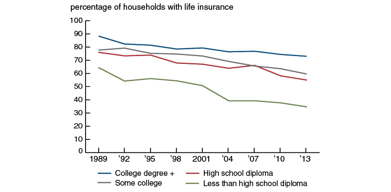
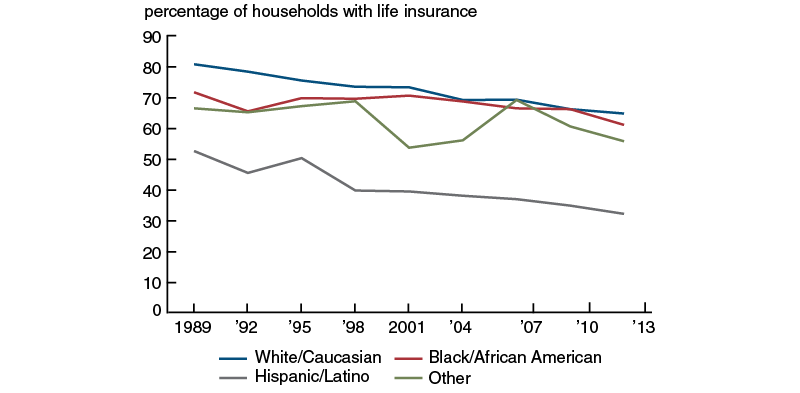
In addition to declining overall, life insurance ownership has declined within each race, education, and income subgroup for both term and cash value products (see figures 2–4, as well as table 3). In percentage terms, the declines have generally been largest among the lower-education and lower-income households for term life products and among the higher-education and lower-income households for cash value products. As a result, the gaps in ownership between high-education and low-education or high-income and low-income households have tended to widen for term life between 1989 and 2013 and shrink for cash value life insurance over the same period. For example, from 1989 to 2013, ownership of term life policies declined by 42 percent among households in the bottom quintile of the income distribution, going from 32.5 percent to 18.8 percent. Among households in the highest income quintile, ownership of term life policies declined by just 0.3 percentage points, from 76 percent to 75.7 percent. As a result of these trends, the gap in ownership rates for term life insurance between the highest income quintile and the lowest income quintile widened from 43.5 percent in 1989 to 56.9 percent in 2013. Over the same period, the gap in ownership of cash value policies for the same groups narrowed from 44.6 percent to 17.3 percent. A large share of this decline is driven by a 53.9 percent decline in the ownership of cash value policies for households in the highest income quintile, with their ownership falling from 57.2 percent in 1989 to 26.4 percent in 2013. Households in the lowest income quintile also saw a drop in their ownership of cash value life insurance, but of a much smaller magnitude in both absolute and percentage terms, with ownership falling from 12.5 percent in 1989 to 9.1 percent in 2013. We see similar patterns when we compare trends in ownership for those without a high school diploma with those who have completed college or more education.
Figure 2. Life insurance ownership by race

Source: Authors’ calculations based on data from the Board of Governors of the Federal Reserve System, Survey of Consumer Finances.
Figure 3. Life insurance by education
Source: Authors’ calculations based on data from the Board of Governors of the Federal Reserve System, Survey of Consumer Finances.
Figure 4. Life insurance by income quintile

Source: Authors’ calculations based on data from the Board of Governors of the Federal Reserve System, Survey of Consumer Finances.
While rates of life insurance ownership have fallen, the face value of policies has increased for both term and cash value insurance. This is the case both in absolute terms and when measured in terms of the number of years of household income represented by the face value of the policy (see table 2). The average face value for term life insurance measured in 2013 dollars climbed from $155,996 in 1989 to $353,288 in 2013, a 126.5 percent increase.8 Over the same period, the average face value for cash value life insurance increased from $157,902 to $225,894, a 43.1 percent increase. The savings component of cash value policies also increased over this period, going from $20,290 in 1989 to $35,896 in 2013, a 76.9 percent increase. We can measure how much insurance coverage has changed from 1989 to 2013 by expressing the face value of policies in terms of the number of years of household income that they represent. To do this, we divide the face value of a policy by household income for each household that has term or cash value life insurance and then average the resulting years over the households with each type of policy. These calculations suggest households with life insurance in 2013 had greater coverage than households in 1989. For term life, the average number of years of income represented by the face value rose from 2.1 in 1989 to 3.3 in 2013. For cash value policies, there was an increase from 2.1 years in 1989 to 2.4 years in 2013. In addition, the average accumulated savings component of a cash value policy rose from 0.24 years in 1989 to 0.36 years in 2013. So while fewer households owned life insurance in 2013 than in 1989, those that did had higher levels of coverage in 2013 than in 1989.
Table 3. Trends by characteristic
|
|
Panel A: Any life insurance | Panel B: Term life insurance | Panel C: Cash value life insurance | |||||||||
|---|---|---|---|---|---|---|---|---|---|---|---|---|
|
|
1989 |
2013 |
Change from |
1989 |
2013 |
Change from |
1989 |
2013 |
Change from
|
|||
|
|
|
|
(% change) |
(level change) |
|
|
(% change) |
(level change) |
|
|
(% change) |
(level change) |
|
Life insurance by race (%) |
||||||||||||
|
White/Caucasian |
80.9 |
64.9 |
–19.7 |
–16.0 |
60.6 |
54.3 |
–10.4 |
–6.3 |
42.5 |
20.7 |
–51.3 |
–21.8 |
|
Black/African American |
71.8 |
61.2 |
–14.8 |
–10.6 |
58.1 |
48.7 |
–16.2 |
–9.4 |
24.3 |
19.1 |
–21.7 |
–5.3 |
|
Hispanic/Latino |
52.7 |
32.3 |
–38.7 |
–20.4 |
39.8 |
28.4 |
–28.8 |
–11.5 |
18.6 |
6.4 |
–65.6 |
–12.2 |
|
Other |
66.6 |
55.9 |
–16.1 |
–10.8 |
56.4 |
47.7 |
–15.3 |
–8.7 |
26.1 |
16.8 |
–35.8 |
–9.3 |
|
White/Caucasian– |
9.1 |
3.8 |
|
|
2.6 |
5.6 |
|
|
18.1 |
1.6 |
|
|
|
White/Caucasian– |
28.2 |
32.6 |
|
|
20.8 |
26.0 |
|
|
23.9 |
14.3 |
|
|
|
Life insurance by education (%) |
||||||||||||
|
Less than high school diploma |
64.4 |
34.7 |
–46.0 |
–29.6 |
44.8 |
28.2 |
–37.0 |
–16.5 |
27.9 |
8.7 |
–68.7 |
–19.2 |
|
High school diploma |
76.0 |
55.0 |
–27.6 |
–21.0 |
57.5 |
44.4 |
–22.7 |
–13.1 |
35.3 |
17.4 |
–50.7 |
–17.9 |
|
Some college |
77.7 |
59.6 |
–23.3 |
–18.1 |
59.3 |
48.8 |
–17.7 |
–10.5 |
40.1 |
19.1 |
–52.3 |
–21.0 |
|
College degree + |
88.3 |
73.0 |
–17.4 |
–15.3 |
71.6 |
62.8 |
–12.2 |
–8.7 |
46.6 |
22.4 |
–51.8 |
–24.2 |
|
Highest education level– |
24.0 |
38.2 |
|
|
26.8 |
34.6 |
|
|
18.7 |
13.7 |
|
|
|
Life insurance by income quintile (%) |
||||||||||||
|
Less than 20 |
43.5 |
26.8 |
–38.4 |
–16.7 |
32.5 |
18.8 |
–42.1 |
–13.7 |
12.5 |
9.1 |
–27.6 |
–3.5 |
|
20–39.9 |
65.1 |
44.5 |
–31.7 |
–20.6 |
46.2 |
35.5 |
–23.0 |
–10.6 |
26.6 |
14.4 |
–45.9 |
–12.2 |
|
40–59.9 |
83.9 |
61.2 |
–27.0 |
–22.7 |
65.5 |
49.9 |
–23.8 |
–15.6 |
35.8 |
17.7 |
–50.5 |
–18.1 |
|
60–79.9 |
90.8 |
77.3 |
–14.8 |
–13.5 |
66.7 |
65.4 |
–2.0 |
–1.3 |
50.0 |
23.9 |
–52.2 |
–26.1 |
|
80–100 |
93.9 |
85.2 |
–9.2 |
–8.7 |
76.0 |
75.7 |
–0.4 |
–0.3 |
57.2 |
26.4 |
–53.9 |
–30.8 |
|
Highest income quintile– |
50.4 |
58.4 |
|
|
43.5 |
56.9 |
|
|
44.6 |
17.3 |
|
|
Source: Authors’ calculations based on 1989 and 2013 data from the Board of Governors of the Federal Reserve System, Survey of Consumer Finances.
Characterizing the demand for life insurance
We characterize the factors associated with life insurance ownership at a point in time using a simple linear regression framework. The dependent and explanatory variables in the analysis are motivated by the literature and summarized in equation 1. We use a linear probability model to estimate the probability that a household owns life insurance. We examine three binary outcome variables: owning any life insurance, owning term life insurance, and owning cash value life insurance. We consider the two types of policies separately for several reasons, including differing trends in ownership, differences in price trajectories highlighted in Brown and Goolsbee (2002), and the likely differences in the motivations associated with purchasing insurance that provides protection only versus one that bundles that protection with a tax-protected investment vehicle.
Specifically, we estimate the following equation:
$$2){{Y}_{i,\,j,\,t}}=~{{\alpha }_{t}}+~{{\beta }_{i,\,j}}{{x}_{i,\,t}}+~{{\varepsilon }_{i,\,j,\,t}}.~$$
The variable \({{Y}_{i,j,t}}\) is equal to one if household i owns life insurance of type j in year t and is zero otherwise. We estimate this equation for two cross sections of data corresponding to t = 1989 and 2013. The explanatory variables included in the vector \({{x}_{i,t}}\) are largely the same as those used in Mulholland, Finke, and Huston (2016) to investigate the decrease in ownership of cash value life insurance. These include: sex, race (we use the SCF categories: white, black, Hispanic, and other), age, age-squared, educational attainment (categories include less than a high school diploma, some college, and college degree or higher), income quintiles, net worth quintiles, an indicator for high net worth (net worth that is greater than or equal to ten times income), an indicator for whether the individual has mortgage, credit card, or other debt (which include loans against pensions, loans against life insurance, margin loans, and miscellaneous loans), an indicator for the presence of children, an indicator for whether the respondent is married, and an indicator for homeownership. These variables are summarized in table 4.
As highlighted in Lewis (1989), life insurance may be purchased as a means to protect dependents from the financial repercussions of the death of the primary earner. For this reason, households with a sole earner or with children might be more likely to purchase life insurance. For households with little wealth, income is expected to play an important role in determining the demand for life insurance since it is likely to be correlated with the amount of household expenses that may remain after the death of the primary earner. A similar relationship may hold between the propensity to own life insurance and wealth. However, at higher levels of wealth, household demand for life insurance may decrease as these households may have sufficient resources to self-insure against the possible loss of future income due to the death of a policyholder, as is implied by equation 1.
Education and financial literacy may help households understand the costs and benefits of life insurance policies, possibly making more-educated and financially literate households more likely to own a policy. In addition, the educational attainment of parents may be an indicator of the expected educational expenses of children. This suggests that more-educated parents may have a higher demand for life insurance so that they ensure that the costs of educating children will be covered, even in the event that one of the parents dies prematurely.
Table 4. Summary statistics
|
|
1989 mean |
1989 median |
2013 mean |
2013 median |
|
Age (years) |
45.19 |
42 |
47.78 |
48 |
|
|
(15.12) |
|
(14.58) |
|
|
Married (%) |
59.82 |
|
59.12 |
|
|
Have children (%) |
50.65 |
|
45.79 |
|
|
Number of children |
1.00 |
1 |
0.88 |
0 |
|
|
(1.22) |
|
(1.17) |
|
|
Male (%) |
73.72 |
|
73.57 |
|
|
Black/African American (%) |
13.05 |
|
15.21 |
|
|
Hispanic/Latino (%) |
8.14 |
|
11.26 |
|
|
Other race (%) |
4.80 |
|
5.02 |
|
|
Years of education |
12.70 |
12 |
13.65 |
14 |
|
|
(3.11) |
|
(2.65) |
|
|
High school diploma (%) |
31.44 |
|
28.92 |
|
|
Some college (%) |
21.19 |
|
24.86 |
|
|
College degree + (%) |
24.43 |
|
35.16 |
|
|
Homeowner (%) |
63.58 |
|
63.59 |
|
|
Renter or other (%) |
36.42 |
|
36.40 |
|
|
Have mortgage, credit, or other debt (%) |
60.99 |
|
63.07 |
|
|
Have IRA account (%) |
26.23 |
|
28.30 |
|
|
Income (2013 $) |
76,293 |
49,024 |
90,700 |
49,712 |
|
|
(311,672) |
|
(387,916) |
|
|
Net worth (2013 $) |
330,680 |
84,142 |
524,279 |
70,200 |
|
|
(1,747,816) |
|
(3,611,244) |
|
|
Net worth ≥ 10x income (%) |
9.12 |
|
9.93 |
|
Source: Authors’ calculations based on 1989 and 2013 data from the Board of Governors of the Federal Reserve System, Survey of Consumer Finances.
Regression results
In table 5, we present estimates from regressions of life insurance ownership on demographic and financial explanatory variables from the 1989 and 2013 SCF surveys. We focus our discussion on the ownership of term and cash value life insurance, specifically on the results shown in columns 3 through 6. Consistent with the theoretical work on the demand for life insurance discussed earlier, we find that married households are more likely to have term life insurance as are households with more education and income (although the specific patterns vary somewhat between 1989 and 2013). In addition, we find that households with a net worth that is at least ten times their income are less likely to own term life insurance. This is consistent with equation 1 and the literature that argues that very wealthy households may have lower demand for insurance because they can self-insure by using their accumulated wealth to cushion the financial impact of a negative shock. Renters appear to be less likely than homeowners to have term life insurance, at least in 2013, and having debt is associated with higher rates of term life insurance ownership in both years.
Table 5. Estimates of equation 2, linear regression results
|
|
Have life insurance (1989) |
Have life insurance (2013) |
Have term life insurance (1989) |
Have term life insurance (2013) |
Have cash value life insurance (1989) |
Have cash value life insurance (2013) |
|
Age |
0.0155** |
0.00493 |
0.0225*** |
0.0154*** |
0.00582 |
–0.00786** |
|
(0.00505) |
(0.00341) |
(0.00562) |
(0.00345) |
(0.00502) |
(0.00277) |
|
|
Age-squared
|
–0.000139** |
–0.0000276 |
–0.000231*** |
–0.000166*** |
–0.0000377 |
0.000119*** |
|
(0.0000526) |
(0.0000361) |
(0.0000593) |
(0.0000370) |
(0.0000532) |
(0.0000306) |
|
|
Married
|
0.121*** |
0.107*** |
0.104** |
0.0771*** |
0.0583 |
0.0565*** |
|
(0.0344) |
(0.0219) |
(0.0388) |
(0.0223) |
(0.0369) |
(0.0163) |
|
|
Have children
|
–0.0143 |
0.0223 |
–0.0271 |
0.0333* |
0.0389 |
0.0101 |
|
(0.0208) |
(0.0154) |
(0.0265) |
(0.0163) |
(0.0257) |
(0.0134) |
|
|
Male
|
–0.0378 |
–0.0717** |
–0.0680 |
–0.0406 |
0.0812* |
–0.0321* |
|
(0.0376) |
(0.0221) |
(0.0396) |
(0.0220) |
(0.0344) |
(0.0163) |
|
|
Black/ |
0.119*** |
0.127*** |
0.126*** |
0.0808*** |
0.0166 |
0.0566** |
|
(0.0311) |
(0.0193) |
(0.0368) |
(0.0207) |
(0.0309) |
(0.0176) |
|
|
Hispanic/Latino
|
–0.126** |
–0.164*** |
–0.0954* |
–0.136*** |
–0.0964** |
–0.0607*** |
|
(0.0424) |
(0.0229) |
(0.0450) |
(0.0231) |
(0.0358) |
(0.0151) |
|
|
Other race |
–0.0529 |
–0.0638* |
0.00992 |
–0.0591 |
–0.0806 |
–0.0145 |
|
(0.0461) |
(0.0324) |
(0.0547) |
(0.0332) |
(0.0474) |
(0.0257) |
|
|
High school diploma |
0.0504 |
0.0549* |
0.0734* |
0.0310 |
0.0175 |
0.0410* |
|
(0.0302) |
(0.0242) |
(0.0337) |
(0.0241) |
(0.0290) |
(0.0172) |
|
|
Some college
|
0.0425 |
0.0872*** |
0.0666 |
0.0587* |
0.0473 |
0.0575** |
|
(0.0339) |
(0.0257) |
(0.0388) |
(0.0257) |
(0.0349) |
(0.0188) |
|
|
College degree + |
0.0750* |
0.110*** |
0.140*** |
0.0975*** |
0.00985 |
0.0429* |
|
(0.0321) |
(0.0265) |
(0.0393) |
(0.0266) |
(0.0363) |
(0.0197) |
|
|
Renter or other |
–0.0372 |
–0.0440* |
–0.0392 |
–0.0654** |
–0.0213 |
0.0116 |
|
(0.0314) |
(0.0208) |
(0.0382) |
(0.0211) |
(0.0357) |
(0.0169) |
|
|
Have mortgage/credit/other debt |
0.124*** |
0.0768*** |
0.0924** |
0.0533** |
0.0905*** |
0.0488*** |
|
(0.0255) |
(0.0164) |
(0.0288) |
(0.0168) |
(0.0255) |
(0.0132) |
|
|
Have IRA or |
0.0596** |
0.0453** |
0.0130 |
0.0503** |
0.0888** |
0.0457** |
|
(0.0190) |
(0.0172) |
(0.0303) |
(0.0187) |
(0.0307) |
(0.0171) |
Table 5 (Continued). Estimates of equation 2, linear regression results
|
|
Have life insurance (1989) |
Have life insurance (2013) |
Have term life insurance (1989) |
Have term life insurance (2013) |
Have cash value life insurance (1989) |
Have cash value life insurance (2013) |
|
Income quintile 2 |
0.144*** |
0.110*** |
0.110** |
0.103*** |
0.0320 |
0.0236 |
|
(0.0400) |
(0.0231) |
(0.0406) |
(0.0224) |
(0.0304) |
(0.0162) |
|
|
Income quintile 3 |
0.239*** |
0.208*** |
0.222*** |
0.187*** |
0.0421 |
0.0236 |
|
(0.0422) |
(0.0249) |
(0.0441) |
(0.0249) |
(0.0370) |
(0.0182) |
|
|
Income quintile 4 |
0.261*** |
0.305*** |
0.192*** |
0.284*** |
0.135** |
0.0524* |
|
(0.0451) |
(0.0270) |
(0.0486) |
(0.0278) |
(0.0422) |
(0.0218) |
|
|
Income quintile 5 |
0.230*** |
0.330*** |
0.256*** |
0.353*** |
0.118* |
0.0292 |
|
(0.0497) |
(0.0307) |
(0.0553) |
(0.0316) |
(0.0484) |
(0.0261) |
|
|
Net worth quintile 2 |
0.130*** |
0.106*** |
0.0736 |
0.0715*** |
0.0895** |
0.0530*** |
|
(0.0385) |
(0.0212) |
(0.0423) |
(0.0210) |
(0.0347) |
(0.0147) |
|
|
Net worth quintile 3 |
0.123** |
0.161*** |
0.0589 |
0.118*** |
0.103* |
0.0723*** |
|
(0.0444) |
(0.0252) |
(0.0511) |
(0.0258) |
(0.0450) |
(0.0198) |
|
|
Net worth quintile 4 |
0.106* |
0.138*** |
0.0256 |
0.0832** |
0.180*** |
0.0826*** |
|
(0.0484) |
(0.0277) |
(0.0567) |
(0.0289) |
(0.0519) |
(0.0236) |
|
|
Net worth quintile 5 |
0.104* |
0.147*** |
0.00540 |
0.0540 |
0.157** |
0.130*** |
|
(0.0526) |
(0.0320) |
(0.0642) |
(0.0340) |
(0.0597) |
(0.0303) |
|
|
Net worth ≥ |
–0.0618 |
–0.0855*** |
–0.128** |
–0.130*** |
0.0689 |
0.0220 |
|
(0.0353) |
(0.0258) |
(0.0432) |
(0.0268) |
(0.0419) |
(0.0261) |
|
|
Constant |
–0.0478 |
–0.00204 |
–0.213 |
–0.169* |
–0.177 |
0.0652 |
|
(0.121) |
(0.0812) |
(0.132) |
(0.0808) |
(0.115) |
(0.0616) |
|
|
Observations |
2,889 |
5,541 |
2,889 |
5,541 |
2,889 |
5,541 |
|
R2 |
0.282 |
0.258 |
0.151 |
0.214 |
0.181 |
0.082 |
|
Adjusted R2 |
0.276 |
0.255 |
0.144 |
0.211 |
0.174 |
0.079 |
Source: Authors’ calculations based on 1989 and 2013 data from the Board of Governors of the Federal Reserve System, Survey of Consumer Finances.
Somewhat surprisingly relative to the predictions of the literature, the presence of children has no significant impact on the likelihood of owning term life insurance. Perhaps the presence of children is not important once all of the other variables are controlled for. Older households are more likely to own term life insurance, although the effect of age diminishes as household heads age. The peak effect of age on term life insurance ownership is about 47 years of age, near the age at which the earnings of an average worker reach their peak as well (Guvenen et al., 2016), consistent with the literature that argues that the demand for life insurance increases with earnings. The regression patterns echo the stark differences in term life insurance ownership across racial groups and suggest that the patterns that we described earlier persist even when other characteristics are controlled for and that differences in insurance ownership are not due simply to differences in observables across racial groups. Black households are between 8 and 13 percentage points more likely to own term life insurance than otherwise similar white households. In contrast, Hispanic households are between 10 and 14 percentage points less likely to own term life insurance than otherwise similar white households.
While the general relationships between the independent variables and the likelihood of owning a term life policy are similar in 1989 and 2013, there are a few differences in the estimates that are worth highlighting. For example, in 1989 households whose heads’ highest educational attainment is a high school diploma are significantly more likely to own term life policies than those who did not complete high school. In 2013, there is no significant difference in ownership between those whose highest level of education is a high school diploma and those who have not completed high school. In addition, term life ownership appears to be more sensitive to net worth and income in 2013 than in 1989. The coefficients on the net worth quintiles are more likely to be significant in the 2013 estimates. Finally, taken together, the dependent variables explain more of the variation in ownership of term life policies in 2013, where the adjusted R-squared is 21.1 percent versus 14.4 percent for the 1989 regression.
Next, we discuss the estimates of the likelihood of owning cash value life insurance in 1989 and 2013. The literature on life insurance ownership speaks less directly to the motivations for owning cash value life insurance, which is both an investment vehicle and a tool for insuring against the financial consequences of death. In contrast to the pattern observed for term life insurance, the explanatory power of the estimates of cash value life insurance ownership is higher in 1989 than in 2013, with an adjusted R-squared of 17.4 percent in 1989 and 7.9 percent in 2013. While the sex of the household head had no significant impact on term life insurance ownership, it is significantly correlated with cash value life insurance ownership. In 1989, male-headed households were 8 percentage points more likely to own cash value life insurance policies than female-headed households. In 2013, we see the opposite, with male-headed households being 3 percentage points less likely to own cash value life insurance. As is the case with term life, black households are more likely to own cash value life insurance and Hispanic households are less likely to own it than otherwise similar white households. The relationship between cash value life insurance ownership and age differs from that of term life. Focusing on the 2013 estimates in which the coefficients on age and age-squared are significant, we see that the likelihood of owning cash value life insurance is a decreasing function of age until about age 35, but it increases thereafter. Education does not play a significant role in determining the ownership of a cash value policy in 1989. However, in 2013 it does, and households whose highest educational attainment is a high school diploma or more are 4–6 percentage points more likely to own a cash value policy than their counterparts who did not complete high school. Relative to the patterns for term life, income plays little role in determining who owns cash value policies, but wealth is strongly correlated with having a cash value policy and wealthier households are more likely to have such a policy, as are households with an IRA or a Keogh account and households who have debts. In contrast to term life, households whose net worth is ten or more times their income are not significantly more likely to have a cash value policy. This finding is consistent with the view that it is possible to use accumulated wealth as a substitute for a term life policy but not for the investment component of a cash value policy.
Oaxaca–Blinder decomposition
To study how much of the change in life insurance ownership between 1989 and 2013 can be explained by the data, we employ a Oaxaca–Blinder decomposition (see Oaxaca, 1973; and Blinder, 1973). After taking expectations, the difference between estimates of equation 1 for 2013 and 1989 can be rearranged to attribute the change in life insurance ownership between 1989 and 2013 to two main factors: differences in the characteristics of the population and differences in the coefficients, or differences in the relationship between these characteristics and the outcomes. For example, one component of the total change in life insurance ownership might be changes in the share of household heads who have completed high school between 1989 and 2013. Another source of change could be changes in how likely high school graduates are to own life insurance in 1989 versus 2013. The first case is an example of a difference that can be attributed to changes in the characteristics of the population between 1989 and 2013: changes in the share of households in various categories—sex, race, age, education, income, net worth, debt, having children, and homeownership status. The second example is a change in life insurance ownership that can be attributed to a change in the estimated coefficients for a given characteristic, or in other words, a change in the prevalence of life insurance ownership within a group that shares a characteristic. The following equation illustrates the linear decomposition:
$$~{{Y}_{13}}-{{Y}_{89}}=\widehat{{{\beta }_{89}}}\left( {{x}_{13}}-{{x}_{89}} \right)+\left( \widehat{{{\beta }_{13}}}-\widehat{{{\beta }_{89}}} \right){{x}_{89}}+\left( \widehat{{{\beta }_{13}}}-\widehat{{{\beta }_{89}}} \right)\left( {{x}_{13}}-{{x}_{89}} \right).$$The first term, \(\widehat{{{\beta }_{89}}}\left( {{x}_{13}}-{{x}_{89}} \right),\) denotes differences attributable to changes in the characteristics of the population (the x values). The second term, \(\left( \widehat{{{\beta }_{13}}}-\widehat{{{\beta }_{89}}} \right){{x}_{89}},\) measures differences due to changes in the relationship between characteristics and the likelihood of owning life insurance (the \(\beta \) values or coefficients). Finally, the third term, \(\left( \widehat{{{\beta }_{13}}}-\widehat{{{\beta }_{89}}} \right)\left( {{x}_{13}}-{{x}_{89}} \right),\) is an interaction term that accounts for the fact that both the explanatory variables and coefficients are changing over the period.9
Figure 5 shows how changes in the demographic and financial characteristics of the population between 1989 and 2013 and changes in the estimated coefficients impact predicted rates of life insurance ownership. The height of the first bar in each group shows the percentage of households who owned life insurance in 1989 and the last bar displays the analogous information for 2013. The height of the second bar corresponds to the share of households that would be predicted to own life insurance if they had 2013 characteristics and the estimated coefficients from 1989. The third bar uses coefficients from 2013 and characteristics from 1989. Comparing the first two bars in each group, it is evident that we would predict a slight increase in insurance ownership between 1989 and 2013, taking into account only the changes in the characteristics of the population and holding the estimated coefficients fixed at their 1989 values. Using the 1989 coefficients, the predicted share of the population that would own life insurance would rise from 76.7 percent in 1989 to 78.4 percent in 2013. Figure 5 shows similar patterns when considering term and cash value life insurance separately. In other words, looking just at the characteristics of the population in 2013 relative to 1989, we would have expected life insurance ownership to rise.10
Of course, this is not what happened. Instead of a slight increase in life insurance ownership, we observe a significant decline. According to our estimates, much of the explanation for this drop is due to changes in the estimated coefficients—or the likelihood that a household with a given characteristic purchases life insurance. This can be seen by comparing the second bar in figure 5 with the fourth bar. The height of the second bar corresponds to the share of 2013 households that would have been predicted to buy life insurance if they behaved like 1989 households. The fourth bar shows the share of 2013 households that actually bought life insurance. The difference in predicted ownership is stark. With 1989 behavior, 78.4 percent of 2013 households would have been predicted to own life insurance; instead the actual prevalence of life insurance ownership among these households is 60.2 percent. We see similar patterns for term and cash value insurance: 60.6 percent predicted ownership versus actual ownership of 50.2 percent for term and for cash value a predicted ownership rate of 38.0 percent and an actual rate of 18.7 percent.
Figure 5. Actual and predicted life insurance ownership

Source: Authors’ calculations based on 1989 and 2013 data from the Board of Governors of the Federal Reserve System, Survey of Consumer Finances.
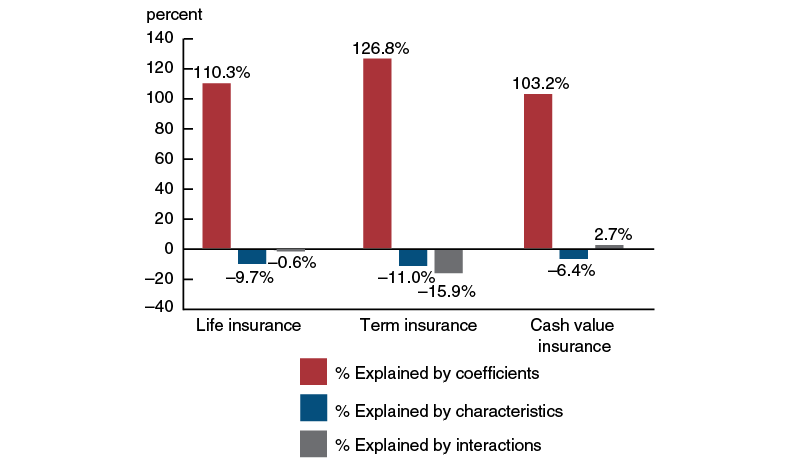
The importance of estimated coefficients relative to changes in characteristics or in the interaction between characteristics and coefficients is demonstrated in figure 6.11 The height of the bars in figure 6 represents the share of the changes in ownership of any life insurance, term life insurance, and cash value life insurance, respectively, that can be explained by changes in the coefficients, changes in demographic or financial characteristics, or by the interaction of the two. The share of the changes in any life insurance ownership and term life insurance ownership that can be explained by changing demographic and financial characteristics and the interaction term is negative, implying that changes in the coefficients must account for more than 100 percent of the change in predicted ownership. The share of the changes in cash value life insurance that can be explained by changes in demographic and financial characteristics, similar to both overall life and term life insurance ownership, is negative. The share of the change in cash value life insurance explained by the interaction term is positive, but near zero. In sum, the decline in life insurance ownership is overwhelmingly driven by changes in the likelihood that an individual with a particular characteristic purchases life insurance.
The results of this exercise are somewhat unsatisfying, in that they tell us that life insurance has gone down because behavior has changed for many households, but they do not tell us much about why that behavior may have changed. We know that if we were to take individuals from 1989 and transport them to 2013, the likelihood that they would own life insurance would have gone down, even if nothing else about them had changed. It is important to recall that our estimates explain only some of the variation in life insurance ownership. Recall that the share of the variation in ownership (the adjusted R-squared) that is explained by the regressions varies from 27.6 percent for owning any life insurance in 1989 to 7.9 percent for owning cash value life insurance in 2013. While these are respectable figures from a statistical perspective, they suggest that much of the story remains to be told.
Figure 6. Percent of outcome gap explained by coefficients, characteristics, and interactions
Source: Authors’ calculations based on 1989 and 2013 data from the Board of Governors of the Federal Reserve System, Survey of Consumer Finances.
Figure 7. Individuals with internet access at home

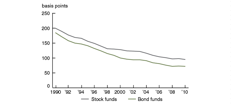
The Oaxaca–Blinder decomposition provides some direction in where we should look for the rest of the story. The fact that the coefficients drive most of the decline in ownership means that we should be looking for trends that might influence the behavior of many households, rather than particular subsets of households. Relevant factors might include trends in the cost of life insurance, how easy it is to purchase, and the availability and cost of substitutes for life insurance (especially relevant for cash value insurance). For example, between 1989 and 2013 internet usage increased dramatically (see figure 7). This would tend to make it easier for households to shop and compare the cost of life insurance from various sources. Brown and Goolsbee (2002) argue that this brought down the cost of term life insurance. Over the same period, the availability and cost of substitutes for the investment component of cash value life insurance, in particular, may have changed. Figure 8 shows a significant decrease in mutual fund fees over this period. In addition, Mulholland, Finke, and Huston (2016) provide evidence that changes in the tax code that created competition for the tax-protected investment features of cash value life insurance may have played a role in the declining demand for this insurance product.
Additional factors that might be important include changes in life expectancy and the extent to which government programs provide insurance against the death of a primary wage earner. Trends in life expectancy are shown in figure 9. The large increase in life expectancy between 1989 and 2013 is likely to play a prominent role in explaining the decline in life insurance ownership over this period. Considerations like those we discussed earlier that influence everyone to varying degrees are challenging to evaluate with cross-sectional data, but they appear to be very important for understanding trends in life insurance ownership. Recent trends in interest rates may also have dampened the demand for cash value life insurance, in particular. The ability to shield investment return from taxes through a cash value life insurance policy is more valuable when nominal returns are higher. When interest rates are low, investment returns, and hence the taxes that might be due on those returns, are lower as well. As a result, the ability to invest through a tax-protected vehicle, such as cash value life insurance, is less valuable in a low interest rate environment.
Figure 8. Mutual fund fees and expenses
Source: Investment Company Institute, 2011, "Trends in the fees and expenses of mutual funds, 2010," ICI Research Perspective, Vol. 17, No. 2, March, available online.
Figure 9. Life expectancy at birth
Conclusion
This article examines trends in life insurance ownership across time and among different types of households. We document substantial differences in the propensity to own life insurance among households with different demographic and socioeconomic characteristics. One fact that stands out is the high life insurance ownership rates of African American households, especially relative to low ownership of other financial assets among these households.
We also investigate the substantial decline in life insurance ownership from 1989 to 2013 and find that households with characteristics that would have made them likely owners of life insurance in 1989 were much less likely to purchase life insurance in 2013. The propensity to purchase life insurance has fallen dramatically across a wide swath of the population since 1989. An interesting pattern emerges when we compare changes in term life insurance ownership and cash value life insurance ownership for high- and low-income households. There has been a substantial drop in term life ownership for low-income households, but only a small decrease in term life ownership for high-income households. We see the opposite pattern for changes in cash value life insurance ownership; it has dropped the least for low-income households and dropped the most for high-income households. That being said, the decline in life insurance ownership is broad-based—showing up across race, education, and income subgroups. This implies that the explanation for the decline in life insurance lies in factors that influence many households rather than just a few. We highlight a few of these trends: changes in life expectancy and changes in factors such as the tax code, internet usage, and mutual fund fees that are likely to influence the price of life insurance as well as the availability of substitutes for the investment component of cash value life insurance. Interesting questions for future research include why life insurance ownership rates for African American households are so high relative to their ownership of other financial assets and how increases in mortality rates for certain demographic groups documented in Case and Deaton (2017) influence the demand for life insurance.
Notes
1 When l = 1, the insurance is actuarially fair, meaning that the present value of the cost of the insurance is equal to the present value of the expected payments under the insurance contract. Insurance is typically sold with a markup, meaning that l is greater than 1 and costs exceed expected payments.
2 Note that when the price of insurance is actuarially fair (l = 1), the term in square brackets equals one and the risk aversion of the dependents plays no role. This is due to the fact that if the price of insurance is actuarially fair, then it is optimal to fully insure, meaning that consumption will be the same in all possible states of the world, eliminating risk.
3 This website, provides a description of the tax treatment of life insurance death benefits.
4 The SCF is conducted every three years. As of the time of our writing, June 2017, the 2013 SCF is the most recent year for which survey data is available.
5 There may be important distinctions in the reasons for purchasing life insurance that is meant to cover end-of-life expenses versus policies that are intended to replace the income of the deceased. Insurers tend to refer to these low-dollar amount face value policies as burial, funeral, or final expense insurance. These policies are offered in both term and cash value varieties. We have repeated all of the analysis in the article with a definition of life insurance ownership that requires the face value of the policy to be greater than the 10th percentile of the face values we observe for each product and each year. This cutoff is $7,256 for term life in 1989, $10,000 in 2013, $7,256 for cash value life insurance in 1989, and $7,000 in 2013. This analysis yields results that are largely the same as what we present here. As a result, we use a definition of life insurance ownership that is equal to one even for policies with a small face value.
6 We use the demographic characteristics of the head of the household to divide households into groups.
7 In fact, our regression estimates in table 5 show that once we control for education, income, wealth, and other characteristics, African Americans are more likely to own life insurance than whites. This may be related to the important role of African American-owned life insurance firms from the early 1920s through the 1960s (Heen, 2009; and Chapin, 2012). Another possible explanation is that higher mortality rates for African Americans make it optimal for more African Americans than whites to choose to own life insurance. However, there is evidence that African Americans, on average, expect to live six years longer than their actuarial life expectancy while whites’ subjective and actuarial life expectancies are much closer (Mirowsky, 1999). We have replicated similar findings using data from the SCF. Studying the reasons for high rates of life insurance ownership among African Americans is an important topic for future research.
8 All dollar figures are reported in real 2013 dollars.
9 We assess the degree to which changes in explanatory variables could account for changes in life insurance ownership if all demographic groups still purchased life insurance at the rate which they did in 1989. One could also consider a similar exercise using the 2013 demographic group life insurance purchasing rates.
10 Note that we come to the same conclusion when we compare the last two bars, which hold the estimated coefficients fixed at their 2013 values. Using 2013 coefficients, we would have expected life insurance ownership to rise from 58.7 percent in 1989 to 60.2 percent in 2013 based on changes in characteristics of the population.
11 It is important to note that this is a decomposition of the variation that is explained by the regression model. For example, the R-squared terms in columns 1 and 2 of table 5 indicate that roughly one-quarter of the variation in the data is explained by the regression model.
REFERENCES
Bernheim, B. Douglas, 1991, “How strong are bequest motives? Evidence based on estimates of the demand for life insurance and annuities,” Journal of Political Economy, Vol. 99, No. 5, October, pp. 899–927.
Blinder, Alan S., 1973, “Wage discrimination: Reduced form and structural estimates,” Journal of Human Resources, Vol. 8, No. 4, Autumn, pp. 436–455.
Board of Governors of the Federal Reserve System, 1989–2013, Survey of Consumer Finances, available online, https://www.federalreserve.gov/econresdata/scf/scfindex.htm, accessed on October 15, 2015.
Brown, Jeffrey R., and Austan Goolsbee, 2002, “Does the internet make markets more competitive? Evidence from the life insurance industry,” Journal of Political Economy, Vol. 110, No. 3, June, pp. 481–507.
Case, Anne, and Angus Deaton, 2017, “Mortality and morbidity in the 21st century,” Brookings Papers on Economic Activity, BPEA Conference Drafts, March 23–24, available online.
Chapin, Christy Ford, 2012, “Going behind with that fifteen cent policy: Black-owned insurance companies and the state,” Journal of Policy History, Vol. 24, No. 4, October, pp. 644–674.
Chen, Renbao, Kie Ann Wong, and Hong Chew Lee, 2001, “Age, period, and cohort effects on life insurance purchases in the U.S.,” Journal of Risk and Insurance, Vol. 68, No. 2, June, pp. 303–327.
Durham, Ashley, 2015, “2015 insurance barometer study,” LIMRA, available online, http://www.orgcorp.com/wp-content/uploads/2015-Insurance-Barometer.pdf, accessed on November 23, 2016.
Fischer, Stanley, 1973, “A life cycle model of life insurance purchases,” International Economic Review, Vol. 14, No. 1, February, pp. 132–152.
Guvenen, Fatih, Fatih Karahan, Serdar Ozkan, and Jae Song, 2016, “What do data on millions of U.S. workers reveal about life-cycle earnings dynamics?,” mimeo, August 3, available online.
Heen, Mary L., 2009, “Ending Jim Crow life insurance rates,” Journal of Law and Social Policy, Vol. 4, No. 2, Fall, pp. 360–399.
Lewis, Frank D., 1989, “Dependents and the demand for life insurance,” American Economic Review, Vol. 79, No. 3, June, pp. 452–467.
Liebenberg, Andre P., James M. Carson, and Randy E. Dumm, 2012, “A dynamic analysis of the demand for life insurance,” Journal of Risk and Insurance, Vol. 79, No. 3, September, pp. 619–644.
Mirowsky, John, 1999, “Subjective life expectancy in the US: Correspondence to actuarial estimates by age, sex and race,” Social Science & Medicine, Vol. 49, No. 7, October, pp. 967–979.
Mulholland, Barry, Michael Finke, and Sandra Huston, 2016, “Understanding the shift in demand for cash value life insurance,” Risk Management and Insurance Review, Vol. 19, No. 1, Spring, pp. 7–36.
Oaxaca, Ronald, 1973, “Male-female wage differentials in urban labor markets, International Economic Review, Vol. 14, No. 3, October, pp. 693–709.
Retzloff, Cheryl D., 2010, “Household trends in U.S. life insurance ownership,” LIMRA, report, November 1, available by subscription, accessed on September 1, 2016.
University of California, Berkeley, and Max Planck Institute for Demographic Research, n.d., The Human Mortality Database, available online, accessed on December 2, 2016.
Yaari, Menahem E., 1965, “Uncertain lifetime, life insurance, and the theory of the consumer,” Review of Economic Studies, Vol. 32, No. 2, April, pp. 137–150.


