

Introduction and summary
Prices have risen significantly across the U.S. economy over the past few years. According to the Consumer Price Index (CPI) from the U.S. Bureau of Labor Statistics (BLS), the price of the basket of goods consumed by the representative household has increased by about 20% since the start of 2021. This increase in prices has been broad-based, impacting products ranging from used cars to fast food, and inflation has been a frequent topic of discussion in the popular press.1 The rapid increase in prices has largely offset growth in personal income, eroding consumer purchasing power and putting downward pressure on consumer sentiment (Gascon and Martorana, 2024). The press releases for the University of Michigan’s Surveys of Consumers have been pointing out since the spring of 2023 that the high levels of prices and associated worsening of affordability have contributed to poor consumer sentiment, even as inflation has fallen and incomes have continued to rise.2
Though they may not be respondents to the Michigan surveys or even representative of the American public, TikTokers and other social media users have also expressed displeasure about the high price levels of homes, cars, and other big-ticket items. A social media trend contending that the U.S. economy is currently in a “Silent Depression” was kicked off in late 2023; by comparing incomes and prices over time, some on social media argue that people are worse off now than during the Great Depression.3 While their comparisons are fraught with problems, the fact that this social media trend exists is emblematic of the economic pessimism and hopelessness among many U.S. consumers as affordability issues persist.
Taken together, the official inflation readings, consumer sentiment surveys, and social media discontent point to the fact that while much of the data and discussion about the rising cost of living is centered around changes in prices and incomes, the levels of prices and incomes are also of interest to the public. Let me illustrate this with an example: When a customer wants to buy a house, they do not input their most recent raise and the most recent house price appreciation in their town into a mortgage calculator; instead, they enter their income level and the price of the home—which are the key variables that constrain a customer’s decision to buy. Thus, when assessing affordability challenges, it is sensible to compare the price levels of goods to the incomes of the consumers purchasing those goods. Understanding how income levels compare with the price levels of goods—especially the price levels of large purchases such as homes and vehicles—helps policymakers quantify and track whether the economy is working for everyone.
When quantifying the affordability of major purchases, economists often choose to focus on the purchasing power of a household. The household is a natural unit of study because it is the level of aggregation where the most expensive financial decisions, such as buying a house, purchasing a car, or financing a college education, typically take place. Affordability metrics often normalize the price of a particular good by the median household income, which gives economists, policymakers, and others an idea of how affordable the good is to the average U.S. household.
While the price levels of houses and cars are available at a high frequency and with a short release lag (between the time the data are realized and the time they are published), this is not the case for household income. The U.S. Bureau of Economic Analysis (BEA) does release each month an estimate of the previous month’s personal income. In theory, this could be scaled by the total number of U.S. households, which is estimated annually, to achieve a mean household income measure. But this is unsatisfying for a couple of reasons. First, this would not account for changes in the number of U.S. households occurring month to month to match the frequency by which the personal income data are reported. Second, the distribution of income is notably right-skewed, as some people have much, much higher incomes than average (that is, the most-extreme income values lie to the right of the mean in the more pronounced tail of the distribution, though the majority of the values lie to the left of the mean). For this reason, median income is more typically cited when discussing affordability. Without any assumptions about the distribution of household income—which itself might change within a given year—economists cannot derive a monthly estimate of median household income from the BEA personal income data release.
The monthly Current Population Survey (CPS) microdata also provide a closer-to-real-time look at median household income. Indeed, the consulting firm Motio Research uses these microdata to construct an index of median household income with approximately the same two-month lag as the CPS itself. While this is certainly a useful measure, it is not entirely suited to my purposes either. Though their methodology is transparent for the most part, the full methodology and the full median household income data series are not publicly available (only the most recent reading of the series appears to be).
The standard measure of annual median household income, from the U.S. Census Bureau, is released every September in the CPS Annual Social and Economic Supplement (ASEC) for the previous year. This once-a-year release, with a lag of about nine months, introduces concerns about the timeliness of statements about affordability, since we can observe increases in the costs of goods before we can observe the changes in the incomes of households. It is precisely when prices are increasing quickly, as they generally have been since 2021, that we would expect incomes to also increase quickly. Yet, without a timely measure of income growth at the household level, it is even more difficult than usual to understand how consumers may be affected. This mismatch makes assessments of affordability difficult to make in near real time, especially during periods of high inflation, when affordability pressures are most salient.
For example, standing in early 2023, with the December 2022 CPI inflation and employment data releases finalized, you would know that prices rose 6.5% on a year-over-year basis and that wages almost kept up, increasing by 6.1% over the same period (based on the Atlanta Fed’s Wage Growth Tracker). While wage growth is a solid indicative measure of how well Americans are “keeping up” with price changes, it does not fully reflect how well the typical household is doing. Wage growth does not include changes in hours per worker or changes to the workforce size, both of which were notable during the Covid-19 pandemic and recovery period. So, if you wanted to know how much the typical household’s income changed over the year 2022, you were out of luck until September 2023. Only after the median household income data in ASEC were published would you learn that the typical household’s income increased by only 5.4%, lagging inflation by even more than wage growth implied.4
In developing a recent article (Gillet and Hull, 2023) about housing affordability, my co-author and I relied on the New York Fed’s Survey of Consumer Expectations as well as the Atlanta Fed’s Wage Growth Tracker (adjusted for changes in hours worked and the employment-to-population ratio) to make comparisons of changes in homebuyer income with changes in median household income. The precision of our estimates was hampered by the lack of transparent and timely data series on median household income. Existing analyses handle this problem in different ways. The National Association of Realtors’ Housing Affordability Index seems to take the U.S. Census Bureau’s median household income reading from the ASEC release at face value. The Atlanta Fed’s Home Ownership Affordability Monitor projects median household income beyond the American Community Survey (ACS) estimates (which I further discuss in the next section), using the latest employment and income data. However, their methodology is not laid out in detail, which makes it difficult to use in other research or policy applications.
Besides being used in analyses of housing affordability, median household income is used in assessing automobile purchases. One example of this use is the Cox Automotive/Moody’s Analytics Vehicle Affordability Index, which expresses the number of weeks of income needed to purchase the average new vehicle. This index uses Moody’s Analytics’ own projections for median household income, which are not publicly available.
Median household income is also of interest in its own right. Tracking growth in real median household income can be a way to monitor whether the typical household is gaining or losing purchasing power. This sort of analysis also suffers from the same data latency issue in the release of the household income data. Motio Research’s real median household income series was launched in late 2023 to address this lack of timely income data. While the other previously mentioned indexes use income as a normalization for the price of a specific good, Motio essentially normalizes income with the cost of the total basket of goods by considering real income. Motio Research’s recent analysis indicates that median household income is of interest and that other analysts take issue with the official government data’s release lags (such as the ASEC data’s release lag). I discuss Motio’s index in greater detail later in this article.
Given the evident demand for a more up-to-date measure of median household income, this article suggests a method for constructing a transparent and accurate forecast of median household income. The proposed method relies only on publicly available, easily accessible data, and it is accompanied by a detailed description and code to allow for replication. My aim with this article is to facilitate closer-to-real-time analysis of affordability and many other economic phenomena related to income.
The resulting measures of year-over-year median household income growth are shown in figure 1, with 50% error bands for the forecasts for 2023 and 2024. Note that the model exactly matches the past data (through 2022) on annual growth in median household income, which is part of its design.
1. Year-over-year growth in median household income: Actual and forecasted, 2015–24
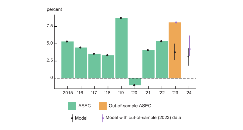
Source: Author’s calculations based on data from the U.S. Census Bureau, Current Population Survey Annual Social and Economic Supplement (ASEC), from ALFRED.
This original forecast, in black in figure 1, was determined entirely by using data up to and including July 2024—obtained from the Federal Reserve Bank of St. Louis’s ALFRED (ArchivaL Federal Reserve Economic Data) database. Thus, the release of ASEC’s 2023 median household income can be considered entirely out-of-sample for this forecast, and I compare it with the model’s forecast in figure 1.5 The model’s forecast of 3.8% growth in 2023 was well below the actual value of 8.0% growth. That said, the model flexibly adapts to the updated information set, and including the 2023 ASEC data point in the model results in a notable upward revision of the anticipated 2024 median household income growth, as shown in purple in figure 1.
So how is this measure created? Though annual household income is only released once per year, with a significant lag, there are income-related variables that cover the same period of interest, but at a higher frequency and with a shorter release lag. As discussed earlier, the BEA’s measure of personal income is released for every month, with about a three-week lag between when the income data are realized and when they are published. So, for instance, by the time September 2024 rolled around and 2023 median household income from ASEC was released, the BEA had released its measure of personal income for every month of 2023 and even seven months of 2024! By carefully considering more up-to-date predictor variables and their historical relationship with the annual income release, I can use statistical methods to construct an estimate of the already realized (but yet-to-be-released) median household income for the previous year. Using known, more-current data to project already realized, but unreleased, data is often referred to as “nowcasting.”
Even after settling on a general framework for tackling the nowcasting problem, there are many choices left to the modeler as to exactly what sort of model to use. I explore a variety of models, including a number of dynamic factor models (DFMs), as a solution to this nowcasting problem. DFMs are well studied in macroeconomic contexts, as in Stock and Watson (2002b), Aruoba, Diebold, and Scotti (2009), and Arias, Gascon, and Rapach (2016). DFMs are often used to combine a (potentially large) set of predictors together, based on the idea that a large fraction of economic variation can be explained by a small set of underlying driving variables. With a series like household income, this assumption seems sensible: A modeler expects that income changes are likely highly correlated to any underlying changes in economic conditions and that this underlying factor can be coaxed out of the predictor variables. DFMs are especially suitable for analysis with real-world data releases, as these models accommodate missing data, different release schedules, different starting dates for predictor series, and mixed frequencies among the included variables.
In the next section, I outline the specifics of the median household income series I forecast, as well as the modeling choices behind the predictor variables I use. Following that section, I describe the details of the nowcasting models further. While many of the modeling details are technical in nature, I aim to provide a detailed intuition for the models I use. I build a baseline dynamic factor model using national U.S. data series and extend that model in ways that balance usability, speed, and accuracy. Utilizing vintage data, I test the baseline model and its extensions in a pseudo-out-of-sample test, similar to what’s done in Stock and Watson (2002b). After this, I analyze the backtesting results, comparing them with the results from other nowcasting models. I conclude this article by selecting a well-performing model specification (whose forecasts are shown in figure 1) and by showing its implications in a housing affordability context, as well as for real household income growth.
Data
In this section, I describe in detail the median household series I will forecast, including its components and its relationship to other measures of income. I also lay out the predictor variables used in the forecast, with rationales for their inclusion.
Prediction target
I seek to build an efficient nowcasting model of median household income. Specifically, within the St. Louis Fed’s FRED (Federal Reserve Economic Data) database, I target the annual series called median household income in the United States (which has the FRED identifier MEHOINUSA646N). This series is released by the U.S. Census Bureau and is derived from the Current Population Survey Annual Social and Economic Supplement. In principle, this same methodology could be used to nowcast the more commonly cited American Community Survey release of median household income, which is also a product of the Census Bureau. The two measures differ as they rely on different survey methodologies, different populations, and different definitions of income.6 Still, the two measures of median household income are quite similar, as seen in figure 2: In panel A, most points lie on or near the 45-degree line, indicating that the two measures are close to each other, and in panel B, the two measures tend to move in tandem over the sample period. Both the ACS and the CPS ASEC are typically released closely together in mid-September,7 so they both have similar significant release lags (of about nine months). Both measures—like the previously mentioned BEA personal income data and monthly CPS income data—reflect similar concepts of income, including employment earnings, income from financial sources (such as interest and dividends), and income from government transfers. I prefer to use the ASEC-based measure for a couple of reasons. First, the ASEC data are available further back in time (from 1984) and have fewer gaps than the ACS data. This allows me to use a longer time series from a single source when fitting the relationships among all the predictors (which I discuss next) and historical household income fluctuations. Second, the ASEC measure is more easily available. It is posted on FRED quickly after release, in September, while the ACS measure (with FRED identifier MHIUS00000A052NCEN) is available on FRED later in the year. I view my choice as one of modeling convenience.
2. Comparison of ACS and ASEC measures of median household income
A. ACS versus ASEC income
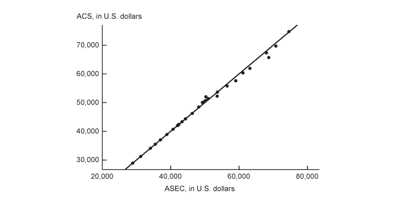
B. ACS and ASEC income, 1984–2024
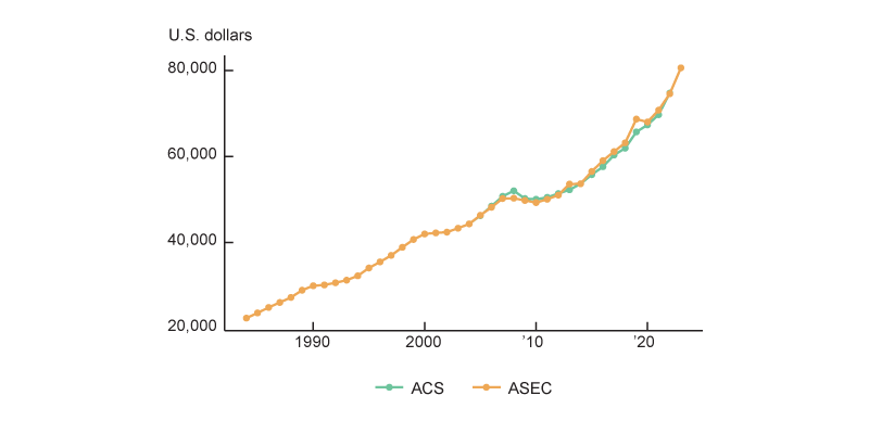
Source: Author’s calculations based on data from the U.S. Census Bureau from FRED.
Predictors
In order to construct my nowcast of median household income, I rely on a panel of 20 series that could plausibly be related to median household income. This set of predictor variables consists of indicators related to labor income, including hourly earnings, hours worked, and the labor force participation rate. I include correlates of other forms of income. For example, I use monthly stock returns and home price appreciation to proxy for income related to capital gains, dividends, and rentals. I also include consumption measures based on the expectation that aggregate spending should be related to aggregate income. In addition, I include the components of the BEA’s release of personal income and outlays data, allowing the model to account for, for example, government transfer payments. By including many income-focused variables in the predictor panel, instead of solely relying on macroeconomic indicators, the latent factors extracted will be more related to income than other parts of the macroeconomy. This selection of predictors is a form of targeting my model to achieve forecasting accuracy for household income. If, for instance, I included many variables related to manufacturing, I might instead capture co-movement in that sector that is less related to household income growth.
Of these 20 predictor variables, 18 of them are monthly; the other two are quarterly. I adjust all series to be approximately stationary. The full list of all series, including their FRED identifiers and the transformations used, are available in figure A1 of the appendix.
Modeling details
The direct inspiration for my suite of models is the Detroit Economic Activity Index, or DEAI (Brave and Traub, 2017; and Brave, Cole, and Traub, 2020). This discontinued Chicago Fed data series leveraged a panel of other Detroit data series to produce a city-specific economic activity index. Notably, the model that produced the DEAI also produced a real per capita income measure for the city in close to real time. I set up a model similar to the DEAI to highlight how to produce a nowcast of annual household income.
In essence, my adaptation posits that a small set of unobserved factor(s) drive the movement of my panel of data series, , which includes both the median household income series of interest and all predictor series. The matrix Z provides the loadings of each of the observed data series onto the factor, so that each of the data series can be described as a linear combination of the common, unobserved factors along with some measurement error, , as in the measurement equation (equation 1). The “dynamics” in the DFM describe the underlying, common factors that are driving the whole data panel as following an autoregressive process with two lags, as outlined in the state equation (equation 2). Here, the and coefficients indicate the reliance of the current value of the state on its previous values, with denoting shocks. The matrices and represent the covariance matrices of the measurement error and the state shocks, respectively. I discuss my choice of lag order in the appendix (see, for example, figures A2 and A3 and the associated discussion).
$\begin{align} 1){\quad}&Y_t=Zf_t+\unicode{x03B5}_t,\\ &\unicode{x03B5}_t∼N(0, H). \end{align}$
$\begin{align} 2){\quad}&f_t = {\unicode{x03C1}_1}{f_{t-1}} + {\unicode{x03C1}_2}{f_{t-2}} + \unicode{x03B7}_t,\\ &\unicode{x03B7}_t∼N(0, Q). \end{align}$
If I knew and , I could in principle obtain an estimate of the whole data panel , including median household income.8
One major stumbling block is that the household income series is an annual series, but I want to include data that are at a quarterly or monthly frequency. I overcome this by using a mixed-frequency model in the style of Mariano and Murasawa (2003), which accommodates monthly, quarterly, and annual series. This augments the simplified set of equations 1 and 2 to enforce that the estimated monthly changes in median household income “add up” to the observed annual fluctuations.
Another major stumbling block is that the household income series is released much later than other series, so it appears missing in our panel for the months before its release date. To accommodate missing data, I estimate this model using the method of Bańbura and Modugno (2014), implemented in the mixed-frequency state space (MFSS) models package in MATLAB from Brave, Butters, and Kelley (2022). I describe the implementation of the estimation procedure in more detail in the appendix.
This allows me to get a monthly glimpse at the household income growth that is consistent with changes in the model’s higher-frequency variables before the low-frequency household income growth is released.
First-order autoregressive errors
One potential improvement to the baseline model that I just described allows the idiosyncratic errors in the series to each follow a stationary autoregressive process with one lag (denoted AR(1)). This improvement is described in Stock and Watson (2011): This model for the idiosyncratic measurement errors posits that the measurement errors are not independent. Instead, there may be variables not captured in the factor model that persistently impact median household income growth, which the persistence in idiosyncratic errors should help account for. The trade-off here is that this adds another parameter to estimate for every series in the panel, which increases estimation time and may induce overfitting. To reduce the number of parameters in the model, I only allow the idiosyncratic errors in the median household income series to have this feature. Thus, the complete model for the household income series and all other predictor series can be written as:$3)\quad\left[ \begin{matrix} {{h}_{t}} \\ {{X}_{t}} \\ \end{matrix} \right]=\left[ \begin{matrix} {{Z}_{h}} \\ {{Z}_{X}} \\ \end{matrix} \right]{{f}_{t}}+\left[ \begin{matrix} \unicode{x03B3} {{\unicode{x03B5} }_{h,t-1}}+{{e}_{h,t}} \\ {{\unicode{x03B5} }_{X,t}} \\ \end{matrix} \right],$
where ${{Y}_{t}}=\left[ \begin{matrix} {{h}_{t}} \\ {{X}_{t}} \\ \end{matrix} \right]$ and $Z=\left[ \begin{matrix} {{Z}_{h}} \\ {{Z}_{X}} \\ \end{matrix} \right].$ This is a similar setup to that in equation 1, but now the measurement errors on the household income series are separated from the measurement errors of the other series. This allows me to have an autocorrelation in the measurement errors for this series, with denoting shocks. Combining equation 3 with equation 2 (the state equation) results in a complete model.
Collapsed factor
In addition to the previous models, I fit a collapsed factor model of the form described by Bräuning and Koopman (2014) and utilized by Brave, Butters, and Kelley (2019). In this type of model, I first “collapse” the panel of predictor variables (which, in this case, does not include household income) using principal components analysis (PCA).9 I model the low-dimensional, unobserved factor(s) extracted from the predictor panel together with the target variable—in this case, median household income. I separate the household income estimation from the predictor series and only use PCA on the predictor panel, , without the target, , in order to approximate . This is represented in equation 5 (shown at the end of this subsection), where the factor has autoregressive dynamics with two lags, as in equation 2.
This system of equations can be obtained by using $\hat{\unicode{x0393} },$ the factor loadings of the static factor model, estimated using PCA. By pre-multiplying the equation by ${\hat{\unicode{x0393} }}'$ (and removing the AR(1) forecast errors for simplicity’s sake), I obtain equation 4:
$4)\quad\left[ \begin{matrix} {{h}_{t}} \\ {\hat{\unicode{x0393} }}'{{X}_{t}} \\ \end{matrix} \right]=\left[ \begin{matrix} {{Z}_{h}} \\ {\hat{\unicode{x0393} }}'{{Z}_{X}} \\ \end{matrix} \right]{{f}_{t}}+\left[ \begin{matrix} {{\unicode{x03B5} }_{h,t}} \\ {\hat{\unicode{x0393} }}'{{\unicode{x03B5} }_{X,t}} \\ \end{matrix} \right].$
However, ${\hat{\unicode{x0393} }}'{{X}_{t}}\equiv {{\hat{f}}_{t}}$ is the principal components estimate of the factor. I take ${\hat{\unicode{x0393} }}'{{\unicode{x03B5} }_{X,t}}\equiv {{\unicode{x03B5} }_{f,t}}$ and set ${\hat{\unicode{x0393} }}'{{Z}_{X}}=I,$where is the identity matrix.10 These simplifications result in equation 5. By applying this step before the model optimization, only the loadings of the household income on the factor need to be estimated, instead of the loadings of all the panel variables. This significantly reduces the number of free parameters in the estimation while, in essence, tilting the extracted factor to match more closely with the desired predicted series, namely, median household income. Because of the narrowly focused predictor series, I am less focused on the use of this collapsed approach to optimally select the factors most explanatory for income changes and more focused on the parsimony of this approach. Equation 5 is a result of this approach:
$5)\quad\left[ \begin{matrix} {{h}_{t}} \\ {{{\hat{f}}}_{t}} \\ \end{matrix} \right]=\left[ \begin{matrix} {{Z}_{h}} \\ I \\ \end{matrix} \right]{{f}_{t}}+\left[ \begin{matrix} {{\unicode{x03B5} }_{h,t}} \\ {{\unicode{x03B5} }_{f,t}} \\ \end{matrix} \right].$
Mixed-frequency vector autoregression
In addition to the dynamic factor models I test, I also test a mixed-frequency vector autoregression (MF-VAR) in the state space framework, inspired by Schorfheide and Song (2015). I use a highly simplified version of their model, without Bayesian estimation methods. The MF-VAR that I use models the evolution of each constituent series, , as dependent on the previous realizations of the same series and those of all other series related to in the panel, . The shocks to each variable are considered orthogonal to each other. This intuition is shown in equation 6, where I combine all into the matrix and all VAR coefficients into the matrix . Note that represents the collection of constant terms for each series.
$\begin{align} 6){\quad}&X_t = c +TX_{t-1} + \unicode{x03B5}_t,\\ &\unicode{x03B5}_t∼N(0, I). \end{align}$
Taking as the vector of time series observed at the annual, quarterly, and monthly frequencies and as the underlying, latent monthly frequency time series, I can write the MF-VAR in state space form, as in equations 7 and 8.11
$7) {\quad} y_t = {Z_t}{s_t},$
$8) {\quad} s_t = {C_t} + {T_t}{s_{t-1}} + {R_t}{\unicode{x03F5}_t}.$
Here, the state vector includes both the latent monthly and the accumulators. These accumulators ensure that the latent properly aggregates to the observed quarterly and annual . These equations are analogous to equations 1 and 2.
Key comparison models
In this subsection, I cover a few models that I use as comparisons for the statistical forecasts of median household income.
Annual autoregression
One straightforward way to construct a statistical forecast of median household income (HHI) would be to fit a simple autoregression to the annual growth in the median household income series, as shown in equation 9. Once the coefficients and are estimated, these coefficients and the most recent log(∆HHIt) reading can be used to create a nowcast.
$9) {\quad} {\mathit{log}}(\unicode{x0394}{HHI_t}) = \unicode{x03B2}_0 + \unicode{x03B2}_1{\mathit{log}}(\unicode{x0394}{HHI_{t-1}}) + \unicode{x03B5}_t.$
Current Population Survey
Unlike all previous models, which provide statistical forecasts of median household income, the monthly release of the Current Population Survey microdata provides a closer-to-real-time look at median household income. As previously mentioned, the consulting firm Motio Research uses these microdata to construct an index of real median household income. However, these monthly CPS microdata would not necessarily match the annual ASEC data, given that the ASEC respondents and questions do not match those of the monthly CPS. Specifically, the monthly CPS asks a single question about which dollar range family income falls into. ASEC asks a series of approximately 50 questions about exact dollar values of specific income sources. The granularity of the monthly CPS microdata also differs from the granularity of ASEC microdata. Monthly CPS family income is reported in about 16 discrete buckets, while annual ASEC household income is reported as a continuous dollar value. At a high level, though, the CPS and ASEC income concepts are similar: Both include income from employment, financial sources, and government transfers.
I follow a procedure similar to that of Motio Research to construct a nominal median household income measure (as opposed to their real median household income measure). This involves interpolating the median from the discrete, weighted count data in IPUMS CPS.12 I seasonally adjust the monthly series and then rebenchmark the index every year based on the latest ASEC release.
This CPS-based series allows me to make a comparison with a data source not included in the other forecasting models. I use this CPS-derived, Motio-inspired index as a point of comparison for my statistical nowcasting methodology.
Backtesting the approach
Ideally, I would evaluate my models with a true out-of-sample test, where I would have developed the nowcasting model in 2012 and let it run, without changes, ever since. Instead, I apply a pseudo-out-of-sample exercise from 2012 through 2022 to understand the nowcasting accuracy of each model. I implement an approach similar to that of Stock and Watson (2002b), where I create nowcasts from my models using only data that would have been released at the time of the nowcast. I leverage the St. Louis Fed’s ALFRED database, which contains vintage economic data.
Through 2022, I retrieve point-in-time data as of just before each year’s ASEC release of the median household income series, sometime in September. Each year, I refit each model. This allows me to get close to the “true” out-of-sample predictions because I account for release lags and data revisions by using as-released data. However, there are some series that do not begin appearing in ALFRED until 2016. In order to extend the backtest over a slightly longer time period, I manually lag each of those series based on its average release lag. This should bring the data closer to point-in-time data, but would not account for data revisions in these few series before 2016.
For each model, I compare each year’s forecast of median household income with the actual released value. I additionally use an average of the models as its own forecasting model. If some models tend to overpredict at the same time that others underpredict, this naive sort of aggregate forecast could perform quite well. The results of this exercise are shown in figure 3.
3. Time series of backtest forecasts and realizations, 2012–22
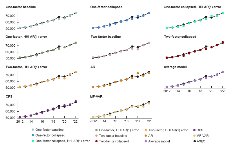
Sources: Author’s calculations based on data from the Federal Reserve Bank of St. Louis, ALFRED; and IPUMS Center for Data Integration, IPUMS CPS.
I see that many models struggled to predict income growth in 2019 and 2020. Given the unprecedented nature of the Covid pandemic and the unprecedented nature of the associated transfer payments, this is unsurprising. Though transfer payments are in the model, they likely were downweighted (through a low loading on the factor) prior to the Covid pandemic. Indeed, government benefits increased from about 16.8% of total personal income in 2019 to 21.3% of total personal income in 2020, according to my calculations using personal income and outlays data from the BEA.
To assess the predictive power of each model, I examine each model’s root mean square error (RMSE) and mean absolute error (MAE) compared with the realized median household income. The RMSE is calculated by taking the square root of the mean squared prediction error, and the MAE is computed by taking the mean of each prediction’s absolute error. Given the squared term, the RMSE tends to overweight outliers compared with the MAE. The pseudo-out-of-sample RMSEs and MAEs are summarized in figure 4. A lower value for these errors represents better forecasting performance. In terms of model performance, my single-factor baseline model performed quite well, and the single-factor model with AR(1) errors in the variables performed slightly better. All models outperformed the naive AR(1) forecast using only household income (note that both RMSE and MAE values for this model are the highest in figure 4)—which indicates that bringing in more real-time indicators related to income is helpful. The baseline statistical model and the model with AR(1) idiosyncratic errors (that is, the one-factor, HHI AR(1) error model in figure 4) do outperform the CPS-based measure, regardless of seasonal adjustments. The best-performing model is an ensemble average of all models in the horse race (see the average model’s panel in figure 3 and its RMSE and MAE values in figure 4)—which indicates that the forecasting errors for the models tend to cancel each other out.
4. Error in forecasting models
| Model | RMSE | MAE |
|---|---|---|
| One-factor baseline | $1,245* | $881* |
| One-factor collapsed | $1,511 | $1,037* |
| One-factor collapsed, HHI AR(1) error | $1,581 | $1,093 |
| One-factor, HHI AR(1) error | $1,198* | $726* |
| Two-factor baseline | $1,487* | $1,018* |
| Two-factor collapsed | $1,494 | $947 |
| Two-factor, HHI AR(1) error | $1,444* | $1,008* |
| AR | $2,174 | $1,456 |
| Average model | $1,160* | $754* |
| CPS | $1,409 | $1,065 |
| MF-VAR | $1,464 | $1,118 |
To this point, I have exclusively focused on the point estimates of the forecast errors, with no consideration for the uncertainty surrounding these forecast errors. To understand whether the outperformance of these forecasts is statistically significant, I first need a benchmark model to evaluate outperformance against. I choose the simple annual AR of household income changes, with one lag, as the benchmark against which to assess outperformance. I apply the Diebold–Mariano test (Diebold and Mariano, 1995) to evaluate whether my model forecasts are significantly more accurate than the annual AR model’s forecasts. This test is robust to forecast errors that are nonnormal and not independently distributed. The results of the Diebold–Mariano test—tested against the alternative that the prediction model is a better forecasting model than the naive annual AR(1)—are shown as asterisks in figure 4. The significance for the RMSEs is based on the squared forecast error, while the significance for the MAEs is based on the absolute forecast error. No prediction model outperforms the basic annual AR(1) model at a 5% significance level, but many models outperform it with marginal significance.
I track the forecast errors over time in figure 5. In this figure with six panels, I show three different ways of computing forecast error. In order to show the Covid-era results without them dominating the scale, I show the errors in the years 2012–19 in the left panels and the errors in the years 2020–22 in the right panels. For each model, the top panels show the raw forecast error, the middle panels show the forecast error as a percent of the realized value, and the bottom panels show the absolute forecast error. Based on the results plotted in figure 5, I see that the accuracy of the model with AR(1) errors is mostly driven by its accuracy in 2020, which was a hard-to-predict year.
5. Time series of errors in forecasting median household income, 2012–22
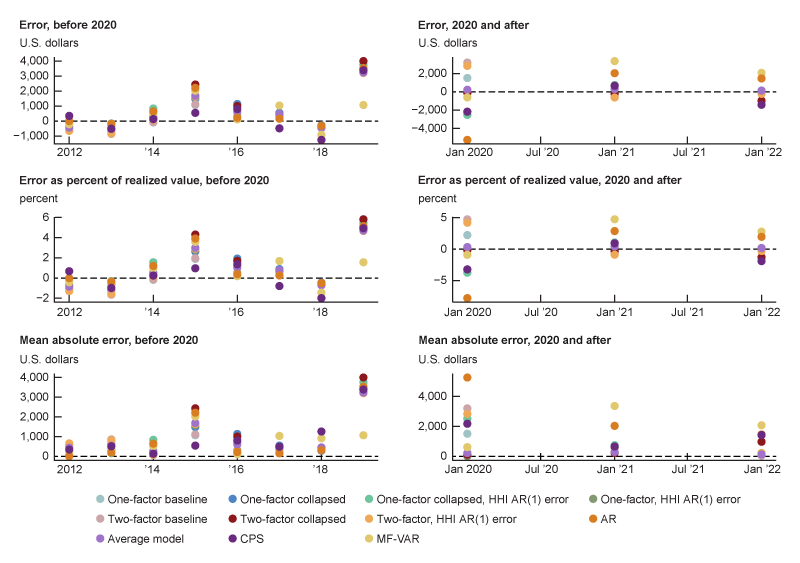
Sources: Author’s calculations based on data from the Federal Reserve Bank of St. Louis, ALFRED; and IPUMS Center for Data Integration, IPUMS CPS.
Estimation time
In the out-of-sample backtesting exercise, I also measure the time to initialize and estimate each model at each forecasting date. The models were initialized and estimated in the Windows 10 version of MATLAB 2022b, using the Parallel Computing Toolbox with an eight-core Intel(R) Core(TM) i7-9700 CPU @ 3.00GHz processor. The estimation times of the models are shown in figure 6. Longer estimation times hinder replicability and quickly make models infeasible to work with. Notably, adding a second factor is fairly time-consuming in terms of estimation time. As expected, the collapsed models greatly reduce the estimation speed because they have fewer parameters to estimate.
6. Estimation (fitting) times of given forecasting models
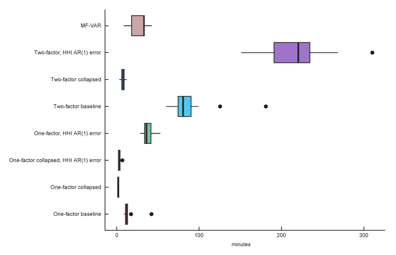
Source: Author’s calculations.
The model with a single factor and AR(1) measurement error for household income (described previously) performs overall the best in my out-of-sample exercise (based on the results of figures 4 and 5) and has a relatively fast estimation time (as shown in figure 6), so it is my preferred model for forecasting median household income.
Applications and extensions
Here, I show a couple of uses for this median household income forecast from my preferred model. I show its utility in assessing home affordability as well as in forecasting household income growth. I then cover some possible improvements and extensions for the model.
Home affordability
I investigate an application of having an updated forecast of annual household income using my preferred single-factor DFM with AR(1) errors. First, I leverage it as a stand-in for the yet-to-be-released ASEC (or ACS) data, which allows me to track home affordability at an annual level, like in Gillet and Hull (2023).13 The ASEC and ACS releases for 2023 income data were released around mid-September 2024. However, before their publication, I was able to estimate home affordability for 2023 with my preferred model’s forecast for median household income. The results are shown in figure 7. I note that in 2023, homes were more unaffordable for a median income household than in any other time in my data set based on my model’s forecasted household income growth for 2023. The actual ASEC value for 2023 median household income growth was higher than the forecast, resulting in a better-than-forecasted picture of affordability. Still, homes were more unaffordable in 2023 than in any other time in the sample.
7. Annual home affordability measure, 2001–23
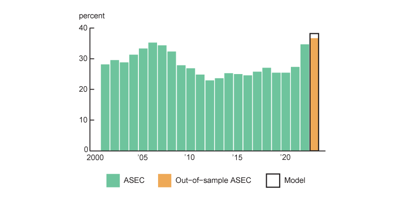
Sources: Author’s calculations based on data from the U.S. Census Bureau, Current Population Survey Annual Social and Economic Supplement (ASEC), from ALFRED; Zillow; Freddie Mac; Fannie Mae; and IPUMS Center for Data Integration, IPUMS USA.
Real household income growth
I take the estimates of year-over-year median household income growth for 2023 and 2024 (estimated before the September 10, 2024, ASEC release) and combine these with the year-over-year changes in the CPI to produce a look at real income growth over the past two years at the household level. For the unknown 2024 CPI inflation rate, I use Wolters Kluwer’s Blue Chip Economic Indicators consensus forecast from July 2024, accessed via Haver Analytics. For comparison, I use the change in the CPS-microdata-based household income measure. I also use the change in real personal income (based on the BEA’s measure) as a benchmark, as I expect household and personal income to have some relationship. These measures are shown since 2019 in figure 8.
8. Growth in real income, 2019–24

Sources: Author’s calculations based on data from the Federal Reserve Bank of St. Louis, ALFRED; IPUMS Center for Data Integration, IPUMS CPS; and Wolters Kluwer, Blue Chip Economic Indicators, from Haver Analytics.
The model-implied real median household income growth shows that 2023 was anticipated to be the first year with positive growth in real median household income since the pandemic hit the United States in early 2020. My model of household income growth projected slightly lower real growth for 2023 than realized in the CPS and BEA data and essentially zero real growth in median household income for 2024. My model’s forecast was well below the realized growth of over 4% in real median household income in 2023, which was released in September 2024. One would expect some divergence between the measure based on BEA data and measures based on the CPS and my model, given that the BEA’s definition of personal income does not map exactly to median household income.14 Additionally, there are differences induced by using a year-over-year measure, like my model produces, and the December-over-December measures shown in the figure, as described in Crump et al. (2014).
Possible extensions
Ideally, I would have a measure of median household income at the monthly frequency. I could then use monthly measures of home prices to make a monthly measure of home affordability. The models as currently implemented provide an interpretable year-over-year income growth measure only once per year, which is useful to nowcast or forecast the U.S. Census Bureau’s CPS ASEC data release for household income, though it does not shed much light on intra-year income dynamics.
One option in the single-factor models would be to calibrate the factor to match the observed mean and standard deviation of household income growth, as in Arias, Gascon, and Rapach (2016) and Clayton-Matthews and Stock (1998)—which would facilitate the interpretation of the factor as monthly household income growth.15 Another approach that I explored was to develop an index in the style of the Chicago Fed Advance Retail Trade Summary, or CARTS (Brave et al., 2021). In this model I benchmarked the factor to exactly fit to the observed annual household income changes. This binding benchmarking is discussed in Durbin and Quenneville (1997). Constraining the annual aggregation of the factor to match the annual change in median household income allows me to use the monthly index as an interpolation of annual household income. Since I already have a monthly index of home prices, I could in theory produce a much more realistic, closer-to-real-time index of home affordability. However, the poor out-of-sample performance of the CARTS-style index precludes its use in this way. In a similar vein, I could rearrange the model matrices so that it would be possible to directly read the monthly income growth from the model.
Another option would be to add the monthly CPS income data into the dynamic factor model. Though this would hurt the model’s replicability and simplicity (as the monthly CPS data are not as easy to acquire as the rest of the data, which are available in FRED), it could be used to help discipline the model and provide a higher-frequency income estimate.
Conclusion
In this article, I describe various models, including some dynamic factor models, with the goal of producing an accurate, closer-to-real-time forecast of median household income. I select a panel of publicly available income-related data and fit a series of proposed models to the data. By running an out-of-sample exercise, I evaluate the models’ performance. I conclude that a single-factor DFM where I model the median household income series to have autocorrelation in its measurement error performs the best and is estimated in a reasonable time. I apply my preferred model to understand changes in housing affordability in 2023, ahead of the U.S. Census Bureau’s September median household income release. I find my preferred model’s forecast of median household income was notably lower than the official median household income value in the CPS ASEC. However, the model flexibly adapts to incoming data and is able to revise upward its forecast for 2024 household income growth. I make my code available in a companion replication packet.
I am grateful for the feedback provided by Gene Amromin, Scott Brave, Marcelo Veracierto, and an anonymous reviewer, as well as the editorial assistance of Han Choi and Julia Baker.
Notes
1 See, for instance, Friedman (2024), Felton (2022), Badkar (2021), and Salvucci (2024).
2 See, for instance, University of Michigan, Office of the Vice President for Communications, Michigan News (2023, 2024).
3 See Dickler (2023) and Kelly (2023).
4 According to monthly personal income measures from the BEA available in early 2023, personal income growth was at 4.5% or 4.8% excluding government transfers—which paints an even dimmer picture of real income growth but tells us something about the change in the average person’s economic well-being, without accounting for household dynamics. As discussed in García and Paciorek (2022), the Covid era was marked by dramatic changes in household arrangements, making the leap from individual-level conclusions to household-level ones more difficult than usual.
5 The CPS ASEC data (including 2023 median household income) were released on September 10, 2024; see U.S. Census Bureau (2024).
6 Full information on the differences between the ACS and CPS ASEC is available in this U.S. Census Bureau fact sheet.
7 For instance, see U.S. Census Bureau (2024), which indicated the income, poverty, and health insurance statistics from CPS ASEC would be released on September 10, 2024, and from the ACS on September 12, 2024.
8 In equations 1 and 2 (and later in equation 6), N indicates normal distribution.
9 See the appendix for a brief description of principal components analysis.
10 This assumption is as in Bräuning and Koopman (2014).
11 This is the notation used in Brave, Butters, and Justiniano (2019); for further details on equations 7 and 8 in my article, consult the discussion about equations 2 and 3 in this reference.
12 Flood et al. (2023).
13 To do this, I take the Zillow Home Value Index on the national level as a stand-in for the typical home price. I can then estimate a typical monthly mortgage payment for a homebuyer of the typical home by using the prevailing Freddie Mac 30-year fixed-rate mortgage average as well as the insurance and tax costs from the ACS—via IPUMS USA (Ruggles et al., 2024)—and Fannie Mae.
14 All of these measures include the most common income sources, such as employment, dividends, and government transfers.
15 Figure A4 in the appendix shows the model state value related to monthly nominal income growth.
Appendix
In this appendix, I provide further details about the modeling approach. First, I explicitly lay out the input data and transformations used in the models. I describe estimation details not covered in the main text, including the basics of principal components analysis and how I selected the lag order for each model. I provide the matrices used in each of the state space models. Finally, I show an example of the nominal income state on a monthly basis.
Data
Here are the data series used in the forecast models.
A1. Data series used in median household income forecast models
| FRED identifier | Description | Transformation |
| MEHOINUSA646N | Median household income | DLN |
| PCE | Personal Consumption Expenditures Price Index | DLN |
| CPIAUCSL | Consumer Price Index (CPI) | DLN |
| CPILFESL | Core CPI | DLN |
| CIVPART | Labor force participation rate | DLV |
| AWHAETP | Average weekly hours of all employees, total private | DLV |
| PAYEMS | All employees, total nonfarm | DLN |
| UNRATE | Unemployment rate | DLV |
| GDP | Gross domestic product | DLN |
| SPASTT01USM661N | Financial market: Share prices for United States | DLN |
| EMRATIO | Employment–population ratio | DLV |
| OPHNFB | Labor productivity | DLN |
| CSUSHPISA | S&P CoreLogic Case-Shiller U.S. National Home Price Index | DLN |
| CES0500000003 | Average hourly private earnings | DLN |
| PI | Personal income | DLN |
| W209RC1 | Received employee compensation | DLN |
| A041RC1 | Proprietor income with adjustments | DLN |
| A048RC1 | Rental income with adjustment | DLN |
| PIROA | Personal income receipts on assets | DLN |
| PCTR | Personal current transfer receipts | DLN |
| TTLHHM156N | Estimate of household count | DLN |
In the backtesting, the equity index used was the Wilshire Total Market Index. However, these data have since been removed from FRED. All analysis using the most up-to-date data instead use this share price measure based on Organisation for Economic Co-operation and Development (OECD) data. Since the models tend to give low weights to this OECD index measure and the two indexes are 97% correlated, I do not anticipate this data change to alter the results of the backtest.
Principal components analysis
In this section, I provide a brief introduction to principal components analysis. Let be an observation of series at time . I assume that each series has been standardized and demeaned. Stacking all series together at a given time gives me the vector , and combining the at all times together gives me a matrix .
I posit that the series have a factor structure; that is, each observation of series at time , , is composed of a linear combination with weights (or loadings) of underlying factors plus some error term :
\[\llap{{{x}_{it}}={{{\unicode{x03B3}}'}_{i}}{{F}_{t}}+{{e}_{it}}}.\]
Or, in matrix form, .
Principal components analysis recovers by an eigendecomposition of the covariance matrix of . The eigenvector corresponding to the largest eigenvalue represents the loadings that transform the first factor into the data, the eigenvector corresponding to the second-largest eigenvalue represents the loadings that transform the second factor into the data, and so on. These factors can be recovered via $F=Γ'X$.
What do these factors mean? The first factor recovered via PCA explains the most variation in the input data series. The second factor is orthogonal to the first factor and explains the most remaining variation in the data, after accounting for the first factor. PCA is often used to reduce the dimensionality of data by extracting only the most meaningful dimensions of the input data, and is shown to provide a consistent estimate of the latent factors, even when the input data have missing observations (Stock and Watson, 2002a).
Lag selection
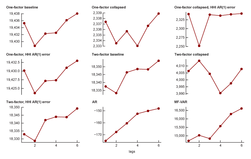
To guide my choice of the lag order to use in my models, I fit each model to the most recent data using one to six lags. I evaluate the fit of each model at these lags and choose one lag for each model type: DFM, MF-VAR, and the annual AR.
In order to evaluate the models, I rely on the Bayesian information criterion, or BIC (Schwarz, 1978), and the Hannan–Quinn information criterion, or HQIC (Hannan and Quinn, 1979). These information criteria are often used for model selection, as they balance the fit of the model against its parsimony to account for the risk of overfitting. Figures A2 and A3 show the BIC and HQIC, respectively, of the fitted model at each of the six lags. For each model, I look for the lag order with the lowest information criteria. For the AR models, this is a lag order of one. For the dynamic factor models, a lag order of two seems more appropriate across the board. For DFMs, this implies that having two months of past data (essentially, the balance of intra-quarter data) is useful. I allow this exercise to guide my choice of lag order, but there are other considerations as well. My criterion for a “good” model is one that forecasts household income well out of sample. If the AR models with a lag order of one and the DFMs with a lag order of two are outclassed in their predictive power by other lag orders, I may choose a higher one. Additionally, I need to consider the time it takes to fit the model to historical data. If a higher lag order is predictive but infeasibly slow to fit, I would not consider it.
A2. BIC at each lag for each model
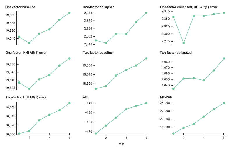
Source: Author’s calculations based on data from the Federal Reserve Bank of St. Louis, ALFRED.
A3. HQIC at each lag for each model
Source: Author’s calculations based on data from the Federal Reserve Bank of St. Louis, ALFRED.
Estimation details
As discussed in the main text, I use the MATLAB MFSS package in order to estimate each type of model. This requires me to put models into state space form as discussed in Brave, Butters, and Kelley (2022), which is similar to the form in Durbin and Koopman (2012).
$\begin{align} \mathrm{A1}){\quad} &y_t = Z_t \unicode{x03B1}_t + d_t + \unicode{x03B2}_t x_t + \unicode{x03B5}_t,\\ &\unicode{x03B5}_t ∼ N(0, H_t). \end{align}$
$\begin{align} \mathrm{A2}){\quad} &\unicode{x03B1}_t = T_t \unicode{x03B1}_{t-1} + c_t + \unicode{x03B3}_t w_t + R_t \unicode{x03B7}_t,\\ &\unicode{x03B7}_t ∼ N(0, Q_t). \end{align}$
This appendix provides further details on these matrices to facilitate setup and estimation. In the following, I assume factors, lags, series, and observations of the series. One approach that I consistently use is putting the requisite lags of in the state matrix, which helps facilitate computation.
I also include some notes on how I initialized the estimation for each of these models.
Baseline model
The following is how I set up the estimation of the baseline model, which is a mixed-frequency dynamic factor model. That is, the following is the matrix setup for the baseline model.
- is an matrix that contains the loadings of the series onto the factors and is padded with zeros to accommodate the lags of .
- is an diagonal matrix. Here, represents the measurement error from the fitting of a single series onto the factors.
- is the identity matrix .
- ensures that the proper variances apply to the states.
- is an matrix. Here, is the ordinary least squares (OLS) VAR coefficient for factor on the th lag of factor . This matrix is structured so that the top portion is the VAR coefficients and the bottom portion ensures that the lagged states are properly accounted for in the state matrix.
$Z=\left[ {{\unicode{x0393} }_{S\times N}}\quad{{0}_{S\times \left( \left( L-1 \right)*N \right)}} \right]\,$,
$H=\left[ \begin{matrix} {{\unicode{x03B5} }_{1}} & {} & 0 \\ {} & \ddots & {} \\ 0 & {} & {{\unicode{x03B5} }_{S}} \\ \end{matrix} \right]\,$,
$R=\left[ \begin{matrix} \begin{align} &{{I}_{N}} \\ &{{0}_{\left( N*\left( L-1 \right) \right)\times \left( N \right)}} \\ \end{align} \end{matrix} \right]\,$,
$T=\left[ \begin{matrix} {{\unicode{x03C1} }_{111}} & \cdots & {{\unicode{x03C1} }_{11N}} & \cdots & {{\unicode{x03C1} }_{L1N}} & \cdots & {{\unicode{x03C1} }_{L1N}} \\ \vdots & \vdots & \vdots & \vdots & \vdots & \vdots & \vdots \\ {{\unicode{x03C1} }_{1N1}} & \cdots & {{\unicode{x03C1} }_{1NN}} & \cdots & {{\unicode{x03C1} }_{LN1}} & \cdots & {{\unicode{x03C1} }_{LNN}} \\ {} & {} & {{I}_{N*\left( L-1 \right)}} & {} & {} & {} & {{0}_{\left( \left( L-1 \right)*N \right)\times N}} \\ \end{matrix} \right]\,$.
I initialize my estimation of the baseline model with and , which is assumed diagonal, extracted using the modified PCA described in appendix A of Stock and Watson (2002b). My initialization of is based on an OLS VAR of the estimated , and is the identity matrix. I follow Doz, Giannone, and Reichlin (2012) in imposing these restrictions on and .
Model with AR(1) errors
The matrix setup for the model with AR(1) errors is similar to that for the baseline model, except I move the measurement error into the state matrix so that the autocorrelation is properly tracked.
- is an matrix that contains the loadings of the series onto the factors and is padded with zeros to accommodate the lags of . The new submatrix compared with the baseline model ensures that the error autocorrelation is incorporated.
- is an diagonal matrix. Here, represents the measurement error from the fitting of a single series onto the factors. Since autocorrelation in the errors of the first series (median household income) is handled in the state, they are treated as zero here.
- represents the innovations in the state and incorporates a term $\unicode{x03C3} _{e}^{2}$ for the innovations in the AR(1) errors.
- ensures that the proper variances apply to the states.
- is an matrix. Here, is the OLS VAR coefficient for factor on the th lag of factor . This matrix is structured so that the top portion is the VAR coefficients and the middle portion ensures that the lagged states are properly accounted for in the state matrix. The bottom portion handles the autocorrelation of the measurement errors with the coefficient .
$Z=\left[ {{\unicode{x0393} }_{S\times N}} \quad {{0}_{S\times \left( \left( L-1 \right)*N \right)}} \quad \begin{matrix} 1 \\ {{0}_{\left( S-1 \right)\times 1}} \\ \end{matrix} \right]\,$,
$H=\left[ \begin{matrix} 0 & 0 & \ldots & 0 \\ 0 & {{\unicode{x03B5} }_{2}} & \ldots & 0 \\ {} & {} & \ddots & {} \\ 0 & {} & {} & {{\unicode{x03B5} }_{S}} \\ \end{matrix} \right]\,$,
$Q=\left[ \begin{matrix} {{I}_{N}} & 0 \\ 0 & \unicode{x03C3} _{e}^{2} \\ \end{matrix} \right]\,$,
$R=\left[ \begin{array}{*{35}{l}} {{I}_{N}} & 0 \\ {{0}_{\left( N*\left( L-1 \right) \right)\times \left( N+1 \right)}} & {} \\ {{0}_{1\times N}} & 1 \\ \end{array} \right]\,$,
$T=\left[ \begin{matrix} {{\unicode{x03C1} }_{111}} & \cdots & {{\unicode{x03C1} }_{11N}} & \cdots & {{\unicode{x03C1} }_{L1N}} & \cdots & {{\unicode{x03C1} }_{L1N}} & 0 \\ \vdots & \vdots & \vdots & \vdots & \vdots & \vdots & \vdots & \vdots \\ {{\unicode{x03C1} }_{1N1}} & \cdots & {{\unicode{x03C1} }_{1NN}} & \cdots & {{\unicode{x03C1} }_{LN1}} & \cdots & {{\unicode{x03C1} }_{LNN}} & 0 \\ {} & {} & {{I}_{N*\left( L-1 \right)}} & {} & {} & {{0}_{\left( \left( L-1 \right)*N \right)\times \left( N+1 \right)}} & {} & {} \\ {} & {} & & {{0}_{1\times \left( N*L \right)}} & {} & {} & {} & {{\unicode{x03C1} }_{\unicode{x03B5} }} \\ \end{matrix} \right]\,$.
In order to initialize and the variance of , I use an OLS VAR on the factor model’s estimate of for the household income series.
Collapsed model
Here is the matrix setup for the collapsed model.
- is an matrix that contains the loadings of the collapsed factors onto the target and is padded with zeros to accommodate the lags of . The bottom portion accommodates the factors.
- is an block-diagonal matrix. Here, $\unicode{x03C3} _{\unicode{x03B5} ,h}^{2}$ represents the variance of the residuals from regressing the target onto the factor. Note that $\unicode{x03C3} _{\unicode{x03B5} ,f}^{2}$ is the variance–covariance matrix of the factors.
- is the identity matrix .
- ensures that the proper variances apply to the states.
- is an matrix. Here, is the OLS VAR coefficient for factor on the th lag of factor . This matrix is structured so that the top portion is the VAR coefficients and the bottom portion ensures that the lagged states are properly accounted for in the state matrix.
$Z=\left[ \begin{matrix} {{\unicode{x0393} }_{1\times N}} & {{0}_{1\times \left( \left( L-1 \right)*N \right)}} \\ {{I}_{N}} & {{0}_{N\times \left( \left( L-1 \right)*N \right)}} \\ \end{matrix} \right]\,$,
$H=\left[ \begin{matrix} \unicode{x03C3} _{\unicode{x03B5} ,h}^{2} & 0 \\ 0 & \unicode{x03C3} _{\unicode{x03B5} ,f}^{2} \\ \end{matrix} \right]\,$,
$R=\left[ \begin{array}{*{35}{l}} {{I}_{N}} \\ {{0}_{\left( N*\left( L-1 \right) \right)\times \left( N \right)}} \\ \end{array} \right]\,$,
$T=\left[ \begin{matrix} {{\unicode{x03C1} }_{111}} & \cdots & {{\unicode{x03C1} }_{11N}} & \cdots & {{\unicode{x03C1} }_{L1N}} & \cdots & {{\unicode{x03C1} }_{L1N}} \\ \vdots & \vdots & \vdots & \vdots & \vdots & \vdots & \vdots \\ {{\unicode{x03C1} }_{1N1}} & \cdots & {{\unicode{x03C1} }_{1NN}} & \cdots & {{\unicode{x03C1} }_{LN1}} & \cdots & {{\unicode{x03C1} }_{LNN}} \\ {} & {} & {{I}_{N*\left( L-1 \right)}} & {} & {} & {{0}_{\left( \left( L-1 \right)*N \right)\times N}} & {} \\ \end{matrix} \right]\,$.
In order to initialize the collapsed model, I need a rough estimate of the high-frequency dynamics of the target household income series to initialize and . To do this, I fit a mixed-frequency VAR to the median household income and the personal income series, which I expect to have similar time-series dynamics. Using this rough initialization of the high-frequency target, I compute the and the error via OLS. Note that is initialized to ten , as a sort of uniform prior on the measurement error in my collapsed factor.
MF-VAR
I use the MFVAR() function in MFSS, which sets up the state space form of the MF-VAR model I specified earlier and estimates it using the expectation–maximization algorithm.
State value related to monthly nominal income growth
Figure A4 shows the value of the state related to monthly nominal income growth, as well as error bands around that state value. Note that the error bands get much wider after June 2024. After this date, the model as fitted does not have any more input data, which increases uncertainty considerably.
A4. State corresponding to monthly change in nominal income, January 2015–June 2025
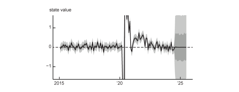
Source: Author’s calculations based on data from the Federal Reserve Bank of St. Louis, ALFRED.
References
Arias, Maria A., Charles S. Gascon, and David E. Rapach, 2016, “Metro business cycles,” Journal of Urban Economics, Vol. 94, July, pp. 90–108. Crossref
Aruoba, S. Borağan, Francis X. Diebold, and Chiara Scotti, 2009, “Real-time measurement of business conditions,” Journal of Business & Economic Statistics, Vol. 27, No. 4, pp. 417–427. Crossref
Badkar, Mamta, 2021, “Record US home prices show signs of cooling,” Financial Times, October 26, available online by subscription.
Bańbura, Marta, and Michele Modugno, 2014, “Maximum likelihood estimation of factor models on datasets with arbitrary pattern of missing data,” Journal of Applied Econometrics, Vol. 29, No. 1, January/February, pp. 133–160. Crossref
Bräuning, Falk, and Siem Jan Koopman, 2014, “Forecasting macroeconomic variables using collapsed dynamic factor analysis,” International Journal of Forecasting, Vol. 30, No. 3, July–September, pp. 572–584. Crossref
Brave, Scott A., R. Andrew Butters, and Alejandro Justiniano, 2019, “Forecasting economic activity with mixed frequency BVARs,” International Journal of Forecasting, Vol. 35, No. 4, October–December, pp. 1692–1707. Crossref
Brave, Scott A., R. Andrew Butters, and David Kelley, 2022, “A practitioner’s guide and MATLAB toolbox for mixed frequency state space models,” Journal of Statistical Software, Vol. 104, No. 10, pp. 1–40. Crossref
Brave, Scott A., R. Andrew Butters, and David Kelley, 2019, “A new ‘big data’ index of U.S. economic activity,” Economic Perspectives, Federal Reserve Bank of Chicago, Vol. 43, No. 1. Crossref
Brave, Scott A., Ross Cole, and Paul Traub, 2020, “Measuring Detroit’s economic progress with the DEAI,” Chicago Fed Letter, Federal Reserve Bank of Chicago, No. 434. Crossref
Brave, Scott A., Michael Fogarty, Daniel Aaronson, Ezra Karger, and Spencer Krane, 2021, “Tracking U.S. consumers in real time with a new weekly index of retail trade,” Federal Reserve Bank of Chicago, working paper, No. 2021-05, revised November 5. Crossref
Brave, Scott A., and Paul Traub, 2017, “Tracking Detroit’s economic recovery after bankruptcy with a new index,” Chicago Fed Letter, Federal Reserve Bank of Chicago, No. 376, available online.
Clayton-Matthews, Alan, and James H. Stock, 1998, “An application of the Stock/Watson index methodology to the Massachusetts economy,” Journal of Economic and Social Measurement, Vol. 25, Nos. 3–4, August, pp. 183–233. Crossref
Crump, Richard K., Stefano Eusepi, David O. Lucca, and Emanuel Moench, 2014, “Data insight: Which growth rate? It’s a weighty subject,” Liberty Street Economics, Federal Reserve Bank of New York, blog, December 29, available online.
Dickler, Jessica, 2023, “Is the U.S. in a ‘silent depression’? Economists weigh in on the viral TikTok theory,” CNBC, December 20, available online.
Diebold, Francis X., and Roberto S. Mariano, 1995, “Comparing predictive accuracy,” Journal of Business & Economic Statistics, Vol. 13, No. 3, pp. 253–263. Crossref
Doz, Catherine, Domenico Giannone, and Lucrezia Reichlin, 2012, “A quasi–maximum likelihood approach for large, approximate dynamic factor models,” Review of Economics and Statistics, Vol. 94, No. 4, November, pp. 1014–1024. Crossref
Durbin, James, and Siem Jan Koopman, 2012, Time Series Analysis by State Space Methods, 2nd ed., Oxford, UK: Oxford University Press. Crossref
Durbin, J., and B. Quenneville, 1997, “Benchmarking by state space models,” International Statistical Review, Vol. 65, No. 1, April, pp. 23–48. Crossref
Felton, Ryan, 2022, “Used-car buyers are seeing relief on once-soaring prices,” Wall Street Journal, May 14, available online by subscription.
Flood, Sarah, Miriam King, Renae Rodgers, Steven Ruggles, J. Robert Warren, Daniel Backman, Annie Chen, Grace Cooper, Stephanie Richards, Megan Schouweiler, and Michael Westberry, 2023, Integrated Public Use Microdata Series, Current Population Survey: Version 11.0, data set, Minneapolis: IPUMS. Crossref
Friedman, Nicole, 2024, “The hidden costs of homeownership are skyrocketing,” Wall Street Journal, April 10, available online by subscription.
García, Daniel, and Andrew Paciorek, 2022, “The remarkable recent rebound in household formation and the prospects for future housing demand,” FEDS Notes, Board of Governors of the Federal Reserve System, May 6. Crossref
Gascon, Charles S., and Joseph Martorana, 2024, “What’s behind the recent slump in consumer sentiment?,” On the Economy Blog, Federal Reserve Bank of St. Louis, January 4, available online.
Gillet, Max, and Cindy Hull, 2023, “Higher home prices and higher rates mean bigger affordability hurdles for the U.S. consumer,” Chicago Fed Letter, Federal Reserve Bank of Chicago, No. 481, August. Crossref
Hannan, E. J., and B. G. Quinn, 1979, “The determination of the order of an autoregression,” Journal of the Royal Statistical Society: Series B (Methodological), Vol. 41, No. 2, January, pp. 190–195. Crossref
Kelly, Jack, 2023, “Viral TikTokers claim the U.S. is in a ‘Silent Depression’ worse than the Great Depression,” Forbes, September 5, available online.
Mariano, Roberto S., and Yasutomo Murasawa, 2003, “A new coincident index of business cycles based on monthly and quarterly series,” Journal of Applied Econometrics, Vol. 18, No. 4, July/August, pp. 427–443. Crossref
Ruggles, Steven, Sarah Flood, Matthew Sobek, Daniel Backman, Annie Chen, Grace Cooper, Stephanie Richards, Renae Rodgers, and Megan Schouweiler, 2024, IPUMS USA: Version 15.0, data set, Minneapolis: IPUMS. Crossref
Salvucci, Jeremy, 2024, “How much have fast-food prices gone up since 2020? Price hikes at 6 popular chains,” TheStreet, June 7, available online.
Schorfheide, Frank, and Dongho Song, 2015, “Real-time forecasting with a mixed-frequency VAR,” Journal of Business & Economic Statistics, Vol. 33, No. 3, pp. 366–380. Crossref
Schwarz, Gideon, 1978, “Estimating the dimension of a model,” Annals of Statistics, Vol. 6, No. 2, March, pp. 461–464. Crossref
Stock, James H., and Mark W. Watson, 2011, “Dynamic factor models,” in The Oxford Handbook of Economic Forecasting, Michael P. Clements and David F. Hendry (eds.), Oxford, UK: Oxford University Press, chapter 2, pp. 35–60. Crossref
Stock, James H., and Mark W. Watson, 2002a, “Forecasting using principal components from a large number of predictors,” Journal of the American Statistical Association, Vol. 97, No. 460, pp. 1167–1179. Crossref
Stock, James H., and Mark W. Watson, 2002b, “Macroeconomic forecasting using diffusion indexes,” Journal of Business & Economic Statistics, Vol. 20, No. 2, pp. 147–162. Crossref
University of Michigan, Office of the Vice President for Communications, Michigan News, 2024, “Consumer sentiment holds steady amid renewed concerns over high prices,” press release, Ann Arbor, MI, April 26, available online.
University of Michigan, Office of the Vice President for Communications, Michigan News, 2023, “Consumer sentiment unmoved amid persistent high prices,” press release, Ann Arbor, MI, April 28, available online.
U.S. Census Bureau, 2024, “Census Bureau releases schedule for income, poverty and health insurance statistics and American Community Survey estimates,” press release, No. CB24-116, Washington, DC, July 16, available online.


