

The following publication has been lightly reedited for spelling, grammar, and style to provide better searchability and an improved reading experience. No substantive changes impacting the data, analysis, or conclusions have been made. A PDF of the originally published version is available here.
This year the sound of corks popping on January 1 not only signaled the dawn of a new year but also the launch of what many have hailed as the most ambitious economic policy of the 20th century, the European Monetary Union (EMU). By joining the EMU, 11 European countries have explicitly agreed to maintain a common monetary policy for an indefinite period. As impressive as this might sound, the 50 states of the U.S. entered into a similar agreement 86 years ago, with the signing of the Federal Reserve Act by President Woodrow Wilson.
There was a great deal of doubt over the long-run viability of the U.S. Federal Reserve System in 1913, largely because it followed two previously unsuccessful attempts at establishing a U.S. central bank.1 Similarly, there is widespread skepticism surrounding the long-run viability of the EMU, although the current debate is more focused, due in large part to Robert Mundell’s seminal work on currency unions, published in the early 1960s.2 Mundell argues that the survival of a currency union depends on how close it comes to the notion of an optimal currency area (OCA). According to this theory, if a monetary union is not an OCA, then some of its members will incur macroeconomic costs (persistent high unemployment and low output) that will outweigh the microeconomic benefits of a single currency (lower transaction and hedging costs), forcing them to abandon the union. Many commentators argue that common monetary policy actions will be damaging to some member countries because the EMU is a long way from an OCA.3
Since Mundell’s work, economists have basically agreed that four criteria must be met for an OCA to exist. First, regions should be exposed to similar sources of economic disturbance (common shocks). Second, the relative importance of these shocks across regions should be similar (symmetric shocks). Third, regions should have similar responses to common shocks (symmetric responses). Finally, if regions are subject to region-specific economic disturbances (idiosyncratic shocks), they need to be capable of quick adjustment. Regions satisfying these criteria will have similar business cycles, so a common monetary policy response would be optimal.
How far the EMU is from an OCA is an open question. At first glance, the data seem to support the skeptics’ view that the EMU is not an OCA. First, EMU countries have experienced frequent and often large idiosyncratic shocks over recent years. A well-known example is German reunification. Second, persistent high unemployment rates throughout Europe suggest that EMU economies are slow to adjust to all economic disturbances.
These observations have spawned a small but growing body of formal empirical research that assesses the long-run viability of potential currency unions. These studies typically approach the issue of whether a region will be a viable monetary union by comparing the region with a well-functioning monetary union (the U.S.) on OCA criteria.4 If the monetary union is as close as the U.S. is to an OCA, then there can be no presumption that it will not be viable in the long run. Alternatively, if the monetary union is less like an OCA than the U.S. is, then there is some doubt about its long-run viability. Implicit in this hypothesis is the critical joint assumption that satisfying OCA criteria is sufficient for a monetary union to be viable and that the U.S. is an OCA. This Chicago Fed Letter examines the usefulness of this research to the EMU debate by summarizing the findings from a recent study that formally investigates whether the U.S. is an OCA.
Do U.S. regions have similar business cycles?
A simple and direct way of making a preliminary assessment of whether the U.S. is an OCA is to calculate the correlation between U.S. aggregate and regional business cycles. A high correlation implies common sources of disturbances and similar responses to disturbances across U.S. regions, while a low correlation indicates differences in the sources of disturbances and/or different responses to disturbances across U.S. regions. I estimate regional cyclical fluctuations by applying a Baxter–King filter to U.S. Department of Commerce, Bureau of Economic Analysis (BEA) quarterly state personal income data from 1969:Q1 to 1998:Q3, deflated by the national Consumer Price Index.5 My estimates suggest that the lowest correlation between a region and the U.S. aggregate is 0.76 for the Southwest, with thftn4e highest at 0.99 for the Southeast. These results suggest that U.S. regions have common sources and responses to disturbances. On the basis of these findings the U.S. cannot be ruled out as an OCA. An obvious weakness of this simple approach is that it does not allow for a comparison of the sources of disturbances or responses to disturbances across regions.
Do U.S. regions have similar sources and responses to disturbances?
One way of overcoming the limitation of the simple business cycle analysis is to use a structural vector autoregression (VAR). A VAR is a statistical method that allows one to estimate how disturbances (or unpredictable changes) to one variable affect other variables in the economy. For example, Carlino and DeFina (1998) use a VAR to jointly estimate the effects of U.S. monetary policy on the 48 contiguous U.S. states (and eight BEA regions).6 Their findings suggest that U.S. monetary policy has a greater impact on more industrial-oriented regions, such as the Great Lakes (they do not provide a formal statistical test of this hypothesis). This implies that the U.S. is not an OCA, since it fails to meet the symmetric response criteria.
My approach to isolating the sources of regional shocks and responses is similar to that used by Carlino and DeFina. I also limit my analysis to the eight BEA regions, but I adopt a slightly different structural model by drawing on the approach of Christiano, Eichenbaum, and Evans in their work on identifying and measuring the aggregate effects of U.S. monetary policy shocks.7 In addition, I break up the analysis by using eight VARs, which estimate the interaction between aggregate U.S. activity and the activity of a given region. Each VAR measures the effect of unpredicted changes in world oil prices, aggregate U.S. income, regional income, and U.S. monetary policy on the region of interest’s income.8 The VARs are estimated using quarterly data from 1969:Q1 to 1998:Q3 (Carlino and DeFina’s data covered 1958:Q1 to 1992:Q4).
With these models in hand, I can assess the similarity of U.S. regional business cycles along two dimensions. First, by studying the sources of regional economic disturbance, I can determine the extent to which fluctuations are caused by common and region-specific shocks. Common shocks include unpredicted changes to world oil prices, aggregate U.S. output, and U.S. monetary policy (U.S. federal funds rate). The relative importance of disturbances is revealed by the one-step-ahead forecast error of regional income. In a perfectly symmetric case, regions would have none of their forecast error explained by region-specific shocks and similar shares for the three common shocks.
Second, by studying the responses to economic disturbances, I can assess whether regions have similar responses to common shocks and determine the time it takes a region to adjust to idiosyncratic shocks. The way a region responds to a shock is revealed through the shape and size of the model’s impulse response function.
Figure 1 reveals that a large share of the disturbance to U.S. regions is due to common shocks (i.e., unexpected shocks to world oil prices, U.S. aggregate income, and U.S. monetary policy). For example, common disturbances explain a large share of the variation in the Southeast, Great Lakes, Mideast, and Far West’s one-step-ahead forecast error (79% to 85%). The Plains and Rocky Mountains appear to have the largest region-specific influences with 53% and 58% of the variation in their one-step-ahead forecast errors explained by common disturbances, respectively. New England and the Southwest fall in between, with common shocks accounting for a little under 70% of the variation in their one-step-ahead forecast error. The relative importance of different common shocks is also similar across regions. Shocks to aggregate U.S. income are a more important source of disturbance than shocks to world oil prices and U.S. monetary policy. Overall, the results suggest that U.S. regions have similar sources of economic disturbances.
1. Variance decompositions for regional income
| Region | Oil Prices | U.S. income | Fed funds rate | Regional income |
| New England | 2 | 67 | 0 | 31 |
| Mideast | 3 | 75 | 1 | 21 |
| Great Lakes | 1 | 80 | 1 | 18 |
| Plains | 2 | 51 | 0 | 47 |
| Southeast | 5 | 80 | 0 | 15 |
| Southwest | 1 | 66 | 0 | 33 |
| Rocky Mountains | 1 | 56 | 1 | 42 |
| Far West | 2 | 79 | 0 | 19 |
Source: Calculations from author’s statistical model, using the following quarterly data series: IMF—world crude oil prices; BEA—personal income by state; and Federal Reserve Board of Governors—federal funds rate.
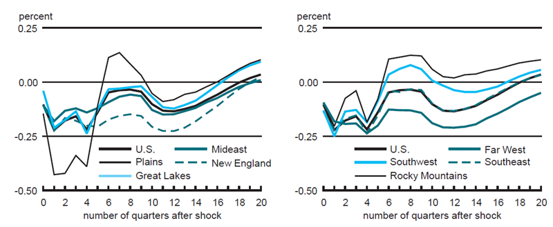
Figures 2–4 describe the responses of the eight BEA regions to common shocks. The lines trace the impulse response functions of regional income: the way regional income responds over time to a one standard deviation shock to world oil prices, aggregate U.S. income, and U.S. monetary policy (U.S. fed funds rate), respectively. In all cases it is clear that the responses of the eight regions are very similar. Figure 2 shows that an unexpected shock to world oil prices has a negative impact on the income of all U.S. regions that dies out after about six quarters. In contrast, figure 3 reveals that an unexpected shock to U.S. aggregate income has a positive impact on all U.S. regions that persists for about six quarters. Finally, figure 4 shows that an unexpected tightening of U.S. monetary policy (an unexpected rise in the U.S. fed funds rate) has a significant negative effect on regional income one and a half to two years after the shock. I also find, like Carlino and DeFina, that unexpected changes in monetary policy seem to have a greater impact on the income of industrial regions, such as the Great Lakes. However, these differences are not statistically significant.
2. Regional output response following shock to world oil prices
Source: Calculations from author’s statistical model, using the following quarterly data series: IMF—world crude oil prices; BEA—personal income by state; and Board of Governors of the Federal Reserve System—federal funds rate.
3. Regional output response following shock to aggregate U.S. income

4. Regional output response following shock to federal funds rate

Turning to region-specific shocks, my model suggests that U.S. regions adjust quickly to idiosyncratic disturbances. The regions can be divided into two groups. First, I find that the responses of the Great Lakes, Plains, Southeast, and Far West to region-specific shocks are not statistically different from zero after about one year. In other words, these regions adjust to idiosyncratic shocks within a year of the initial disturbance. Second, New England, Mideast, Southwest, and Rocky Mountains take about three years to adjust to region-specific shocks. They have responses to idiosyncratic shocks that are not statistically different from zero after about three years.
Conclusion
Much of the skepticism surrounding the long-run viability of the EMU is based on the belief that the monetary union is a long way from an OCA. Evidence supporting this view comes from empirical research that compares the EMU to the U.S. on critical OCA criteria. A key assumption underlying this approach is that the U.S. is an OCA. Evidence presented here suggests that U.S. economic regions do satisfy OCA criteria. In particular, U.S. regions have highly correlated business cycles that are the product of similar cycles of economic disturbance and similar responses to these disturbances. A highlight of these results is that the estimated effects of U.S. monetary policy are similar in all U.S. regions.
Tracking Midwest manufacturing activity
Manufacturing output indexes (1992=100)
| July | Month ago | Year ago | |
|---|---|---|---|
| CFMMI | 132.1 | 131.1 | 124.5 |
| IP | 139.4 | 138.6 | 133.6 |
Motor vehicle production (millions, seasonally adj. annual rate)
| August | Month ago | Year ago | |
|---|---|---|---|
| Cars | 5.8 | 5.4 | 6.3 |
| Light trucks | 7.7 | 6.7 | 6.6 |
Purchasing managers' surveys: net % reporting production growth
| August | Month ago | Year ago | |
|---|---|---|---|
| MW | 54.2 | 62.2 | 59.3 |
| U.S. | 56.7 | 58.2 | 50.3 |
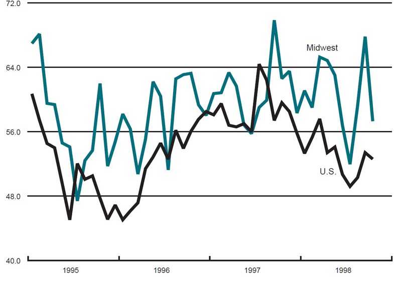
Purchasing managers' surveys (production index)
Light truck production increased from 6.7 million units in July to 7.7 million units in August and car production increased from 5.4 million units in July to 5.8 million units in August. The Chicago Fed Midwest Manufacturing Index (CFMMI) rose 0.7% in July following a 0.5% gain in June. By comparison, the national Industrial Production Index (IP) for manufacturing increased 0.6% in July and 0.1% in June.
The Midwest purchasing managers’ composite index for production decreased to 54.2% in August from 62.2% in July. The purchasing managers’ indexes decreased for Chicago and Detroit but increased for Milwaukee. The national purchasing managers’ survey for production also decreased from 58.2% to 56.7% from July to August.
Notes
1 The First Bank of the United States was disbanded in 1811, and the national charter of the Second Bank of the United States expired in 1836 after its renewal had been vetoed by President Andrew Jackson.
2 See, R. A. Mundell, 1961, “A theory of optimum currency areas,” American Economic Review, Vol. 51, pp. 657–665.
3 See, for example, “Euro brief: The merits of one money,” The Economist, October 28, 1998, pp. 85–86.
4 See M. A. Kouparitsas, 1999, “Is the EMU a viable common currency area? A VAR analysis of regional business cycles,” Federal Reserve Bank of Chicago, Economic Perspectives, Vol. 23, Fourth Quarter, forthcoming, and references therein.
5 See M. Baxter and R. G. King, 1995, “Measuring business cycles: Approximate band pass filters for economic time series,” National Bureau of Economic Research, working paper, No. 5022.
6 See G. A. Carlino and R. DeFina, 1998, “The differential regional effects of monetary policy,” The Review of Economics and Statistics, Vol. 80, pp. 572–587.
7 See L. J. Christiano, M. Eichenbaum, and C. L. Evans, 1994, “Identification and the effects of monetary policy shocks,” Federal Reserve Bank of Chicago, working paper, No. 94–7.
8 Kouparitsas, op. cit.


