

The following publication has been lightly reedited for spelling, grammar, and style to provide better searchability and an improved reading experience. No substantive changes impacting the data, analysis, or conclusions have been made. A PDF of the originally published version is available here.
Recent research on the transmission of economic status from one generation to the next suggests that the persistence in inequality is about 50% higher than previously thought. While the underlying factors that cause substantial immobility in the U.S. remain poorly understood, borrowing constraints among families with low net worth may play a role in perpetuating inequality.
How economically mobile is the United States? Do all children have the opportunity to achieve economic success irrespective of their economic circumstances at birth? Is there an economic underclass that is essentially trapped in poverty for generations? The answers to these questions undoubtedly have a bearing on whether America should be viewed as an equal opportunity society and whether additional policies are needed to address long-term inequities. Despite the obvious importance of economic mobility in determining public policies, economists have only recently begun to carefully study the dynamics of inequality among families over generations.
Several studies undertaken in the 1990s found a relatively high degree of transmission of economic status from fathers to sons, suggesting that the U.S. is not nearly as mobile a society as many had previously thought. For example, the results implied that about 40% of the gap in earnings between Black and White men would persist from one generation to the next—roughly twice the rate of persistence that previous research had found.
Although these studies used substantially better data than previous work, they still suffer from a number of limitations that have the effect of underestimating the degree of intergenerational persistence in inequality. In this Chicago Fed Letter, I describe the results of recent research that suggests that the persistence in inequality is about 50% higher than the consensus view among economists. Although the underlying factors that cause substantial immobility in the U.S. remain poorly understood, some preliminary work suggests that borrowing constraints among families with low net worth may play a role in perpetuating inequality.
The Galton model
Beginning with Sir Francis Galton in the nineteenth century, researchers have tried to measure the rate of regression to the mean of particular characteristics across generations. In a famous example, Galton (1889) plotted the height of adults against their parents’ height and calculated the slope of the line that best fit the data.1 Galton found that, on average, the height of children was about two-thirds that of their parents. Sociologists were the first to apply this type of statistical model to characterize intergenerational inequality by calculating the correlation of various measures of socioeconomic status across generations.
In recent decades, economists have begun to use the Galton model on more traditional economic measures such as wages and annual earnings. Essentially, this involves using ordinary least squares (OLS) to regress the log of the child’s adult earnings on the log of the parent’s earnings. Typically, studies have focused on fathers and sons. The estimated coefficient, r, is referred to as the intergenerational elasticity and almost always takes on a value between 0 and 1.
An intergenerational elasticity of exactly 1 would imply an extremely rigid society, where the son’s position in the earnings distribution would simply replicate his father’s position in the previous generation. In contrast, an intergenerational elasticity of 0 suggests an extremely mobile society in which the son’s earnings are essentially unrelated to his father’s earnings. Values between 0 and 1 provide a useful gauge of the degree of economic rigidity in society. One minus r, on the other hand, provides a measure of the degree to which earnings “regress” toward the mean and can be viewed as a measure of mobility. Therefore, a society with a high r may be seen as a less mobile society than one with a low r.
One useful way to illustrate the quantitative significance of this measure is to imagine what it implies about the evolution of the Black–White wage gap in the U.S. An intergenerational elasticity of 0.2, for instance, implies that only 20% of any earnings gap between groups would remain after a generation (say 25 years).2 Using this logic, the Black–White wage differential for young men that stood at about 25% in 1980 would be reduced to just 5% by 2005. If instead, the intergenerational coefficient were 0.6, then the Black–White wage gap would still be a sizable 15% in 2005. This measure is also useful in thinking about other important issues such as the persistence of poverty, the rate of assimilation of immigrants, and the second-generation effects of income policies.
It’s all in the measurement
To successfully estimate the Galton model, we need good measures of economic status for two generations of individuals from the same family for a large, nationally representative sample. What is especially important is the number of years used to measure economic status. For a variety of reasons, such as layoffs, promotions, and job switching, individual earnings in any particular year contain a sizable “transitory” component that makes this a rather noisy measure of an individual’s lifetime economic status. This is especially true for people who are very young or very old. Therefore, it is crucial to measure “permanent” economic status by averaging information over long periods. In the context of a regression model, it is particularly important to accurately measure the lifetime economic status of the fathers. Since this is a right-hand-side variable, mismeasurement will actually lead to estimates of the intergenerational elasticity that are biased downwards.
In the early 1990s, the first studies to use nationally representative longitudinal datasets, such as the Panel Study of Income Dynamics (PSID) and the National Longitudinal Surveys (NLS), found that averaging a few years of income made a dramatic difference to the results. These studies found the intergenerational elasticity to be about 0.4, roughly twice the estimates of previous studies that had only used single measures of income on unrepresentative samples.
These datasets, however, are still far from ideal for measuring the intergenerational elasticity. The key problem is that many individuals in these surveys tend to drop out of the sample over time for various reasons. This not only reduces the sample size but also requires researchers to use relatively short windows of time over which to measure lifetime economic status. Typically, researchers have used only up to five-year averages of fathers’ income in estimating the Galton model. But does this really make such a big difference? There is reason to believe that it does. This is because many transitory shocks to income, say due to a recession or a health problem, tend to persist for a few years. If averages are taken over short time horizons, then these shocks are not averaged away.
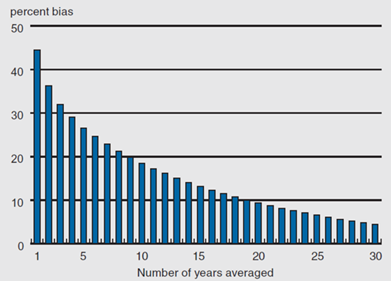
In order to get a sense of how this might affect estimates of r, I conducted simulations using assumptions about the “time series” properties of earnings. Since the 1970s, labor economists have conducted studies on earnings dynamics where they have identified how much of the variance of earnings in a single year is transitory versus permanent and how persistent these transitory fluctuations tend to be from year to year. I incorporated the estimates from these models to determine the amount of downward bias that results from using a short-term average of income as a proxy for life-time earnings.
The results are shown in figure 1. The horizontal axis represents the number of years over which a father’s earnings are averaged and the vertical axis plots the amount of downward bias in the estimate of the intergenerational elasticity. So, for example, using just a single year of earnings results in a coefficient that is biased down by about 45%. As averages are taken over longer periods this bias drops considerably. However, it is clear that even a five-year average can result in an estimate that is biased downward by about 27%. Therefore, an estimate of 0.4 obtained using a five-year average implies that the “true” r is between 0.5 and 0.6 —suggesting substantial intergenerational immobility.
1. Implied bias in intergenerational elasticity
New estimates of intergenerational inequality
Ideally, the most direct way to obtain accurate estimates of the intergenerational elasticity would be to actually use a sample that has the long-term earnings histories of fathers and sons. In fact, a confidential dataset that matches fathers and sons in the Census Bureau’s 1984 Survey of Income and Program Participation (SIPP) to their social security earnings records from 1951 to 1998 was used for exactly this purpose.3 The earnings of sons were averaged from 1995 to 1998 when they were in their early thirties and the earnings of the fathers were averaged over various periods ending in 1985. The results are shown in figure 2.
2. Estimated intergenerational elasticity
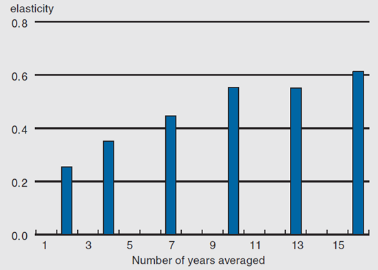
As was the case in earlier studies, the estimate of r is close to 0.4 when using only four-year averages of fathers’ earnings. However, when earnings are averaged over as many as 16 years, the estimate is slightly greater than 0.6. It appears that it is the greater window over which the lifetime economic status of fathers is measured that is the key factor.
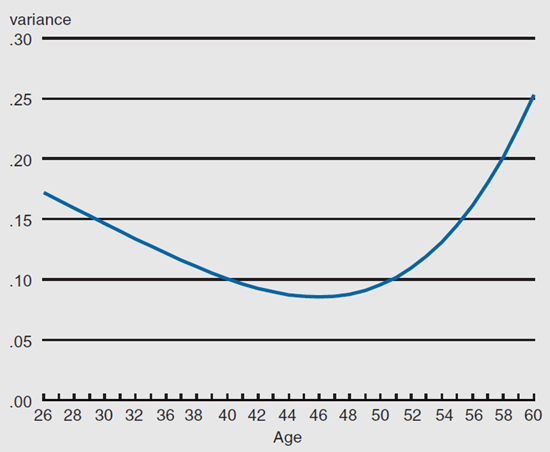
Another possible explanation for this result is that the age at which fathers’ earnings are measured might matter. If younger or older fathers have especially volatile earnings, then averaging their earnings over periods in which their earnings are more stable might lead to less biased estimates. In order to test this hypothesis, I estimated an earnings dynamics model that incorporated age effects to uncover the life-cycle pattern of the transitory variance in log earnings. The results do, in fact, show a pronounced U-shaped pattern to the variance of transitory fluctuations, as we see in figure 3.
3. Lifecycle pattern of variance of transitory shocks
Given their relatively small samples, previous research that used the PSID and NLS might have relied too heavily on families with fathers who were especially young or old. Therefore, I reexamined the results from one highly influential study using the PSID (Solon, 1992) employing a new econometric procedure that essentially weights observations by their estimated reliability based on the age of the fathers.4 The effect of incorporating these age effects was to change the estimate of r from 0.413 to 0.620.
Given that three different approaches have all produced the same result—that the intergenerational elasticity in earnings is about 0.6—strongly suggests that the previous consensus view of 0.4 should be revised upwards. Although it is difficult to make comparisons across countries in intergenerational mobility due to methodological differences, the results for the U.S. appear to be significantly higher than what has been found in other industrialized countries. For example, a similar study using tax records for a very large sample in Canada found an intergenerational elasticity of about 0.2.5 This suggests that the U.S. is not very economically mobile and that further policies might be in order to promote equal opportunity.
Does money matter?
Although the intergenerational elasticity in earnings appears to be quite high, the underlying channels through which economic advantages are transmitted from parents to children are not well understood. Social scientists have proposed a number of explanations including genetically transmitted ability, parents’ investment in their children’s human capital, the implicit or explicit transmission of valuable social networks and social capital, or the high propensity of sons to have the same occupation as fathers. Obviously, it will be difficult to design appropriate policies without a better understanding of which factors are at work.
For economists, the well-developed theory of human capital is an obvious starting point. These theoretical models typically predict that under ideal market conditions the intergenerational elasticity should be quite low, since parents will optimally choose the appropriate level of “investment” in their child’s schooling irrespective of their own financial conditions. However, in the presence of credit constraints, low-income families with “high-potential” children might underinvest in their children’s schooling, thereby inducing a sizable correlation in economic status across generations.
Using the intergenerational sample drawn from the SIPP described earlier, I tested this hypothesis by comparing the intergenerational elasticity for families from different parts of the wealth distribution. Indeed, those in the bottom quartile of net worth had a sharply higher estimated coefficient than those in the top quartile, and the difference was statistically significant. This provides some preliminary evidence that borrowing constraints may be an important factor in the intergenerational persistence of income.
This is an important result because a number of studies have been unable to identify any causal effect of family income on children’s future success. This has led some to argue that money itself does not matter but rather it is other family characteristics associated with income, such as motivation, that are driving the intergenerational association in income. However, these studies typically have not focused on families with little or no wealth. If money matters, but primarily for families that are unable to borrow against future income, then this might help explain the puzzle.
Still, there is considerably more that we need to understand about borrowing constraints before successful policies can be developed. For example, is the lack of access to credit mainly a problem for students at the time of going to college, or is it a deeper problem that affects the quality of schooling at much younger ages? It might be that families with limited financial resources are unable to “buy” into the neighborhoods with the best schools.
Conclusion
Recent research that has measured the intergenerational elasticity in earnings between fathers and their children shows that there is a substantial degree of persistence in income among families over generations. These studies suggest that the rise in income inequality in recent decades may persist for several generations. The underlying mechanisms that enable this persistence are not well understood. However, recent research suggests that the existence of borrowing constraints among those with little wealth is a plausible candidate to explain the high intergenerational elasticity. Families that are unable to access credit may not optimally invest in their children’s schooling. Gaining a better understanding of the nature of these borrowing constraints is a necessary step in designing the appropriate policies to foster greater income mobility.
Notes
1 Francis Galton, 1889, Natural Inheritance, London: Macmillan, p. 97.
2 This example assumes a common intergenerational elasticity for both groups and no other group-specific effects. For example, a number of factors such as skill-biased technical change or declining unionism could affect each group differently and temporarily widen the gap further.
3 See Bhashkar Mazumder, 2001, “Earnings mobility in the US: A new look at intergenerational inequality,” Federal Reserve Bank of Chicago, working paper, No. 2001-18.
4 See Gary Solon, 1992, “Intergenerational income mobility in the United States,” American Economic Review, Vol. 82, pp. 393–408. See also Daniel G. Sullivan, 2001, “A note on the estimation of linear regression models with heteroscedastic measurement errors,” Federal Reserve Bank of Chicago, working paper, No. 2001-23, for more detail on the econometric procedure that was used.
5 See Miles Corak and Andrew Heisz, 1999, “The intergenerational earnings and income mobility of Canadian men: Evidence from longitudinal income tax data,” Journal of Human Resources, Vol. 34, No. 3, pp. 504–533.


