The recent conflict in the Middle East has led to a spike in oil prices, with the potential for production disruptions in the U.S. economy. In this Chicago Fed Letter, we perform a simple share-based calculation to assess the potential effect of the 2026 oil price shock on U.S. gross domestic product (GDP). We apply a sufficient statistics approach that relates the impact on GDP to 1) the oil “domestic absorption ratio,” i.e., the ratio of nominal gross domestic absorption of oil (which we explain in detail in the next section) to nominal GDP and 2) the change in this ratio in response to the shock. Contrary to common wisdom, the domestic absorption ratio is roughly the same today as in the early 1970s, despite a large decline in the real use of oil. The shares approach generally yields modest effects of the 2026 oil price shock, e.g., a change of around –0.17% in GDP in our baseline example calibrated with a 50% increase in the price of oil. An upper bound of the reduction using the shares approach is likely around –0.83%. The approach assumes wages and prices are completely flexible, and it does not account for a potential increase in domestic oil production in response to the shock. Relaxing the former would likely increase the estimated GDP impacts, while relaxing the latter would lower them.
The share of oil in the U.S. economy
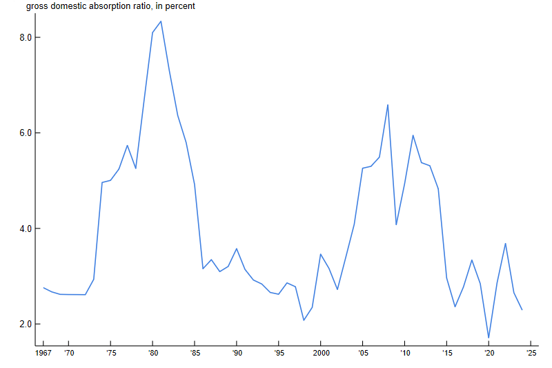
Figure 1 plots nominal gross domestic absorption of oil as a fraction of nominal GDP, which we term the “domestic absorption ratio” or the “oil share.” This is the relevant share to assess the potential impact of the oil shock on domestic output. We measure gross domestic absorption using data from the U.S. Bureau of Economic Analysis's (BEA) Input-Output Accounts on the output of two sectors related to oil: 1) petroleum and coal products (petroleum sector) and 2) oil and gas extraction (extraction sector).1
1. The oil share in the U.S. economy, 1967–2024
Sources: Authors’ calculations based on data from the U.S. Bureau of Economic Analysis, Input-Output Accounts and National Income and Product Accounts of the United States, from Haver Analytics and FRED.
To compute the domestic absorption ratio, first, we take total (gross) output of petroleum, add imports, and subtract exports of the same. This calculation yields gross domestic absorption of petroleum and includes the output of the extraction sector that is sold to the petroleum sector, which in recent years has been roughly 75% of extraction sector output, according to our calculations using BEA data. In a second step, we add to petroleum absorption the value of the extraction sector’s gross output that is used in sectors of the economy other than the petroleum sector. We calculate this value as the total use of extraction sector output as an intermediate input across all sectors minus the use of extraction sector output by the petroleum sector (there is no final use of extraction sector output). Adding this to gross domestic absorption of the petroleum sector yields total gross domestic absorption of oil-related products in the U.S. economy.
Our gross domestic absorption measure captures both domestic final use of oil and use of oil as an intermediate input into domestic production of other goods and services; the oil may be produced domestically or imported. Dividing this value by nominal GDP yields the domestic absorption ratio.
Figure 1 shows, perhaps surprisingly, that at around 2.5% in recent years, the domestic absorption ratio is not much different from its level in the late 1960s and early 1970s.2 Furthermore, the domestic absorption ratio exhibits significant fluctuations; for instance, the absorption ratio increased by roughly 5.5 percentage points during the late 1970s and early 1980s before falling rapidly.
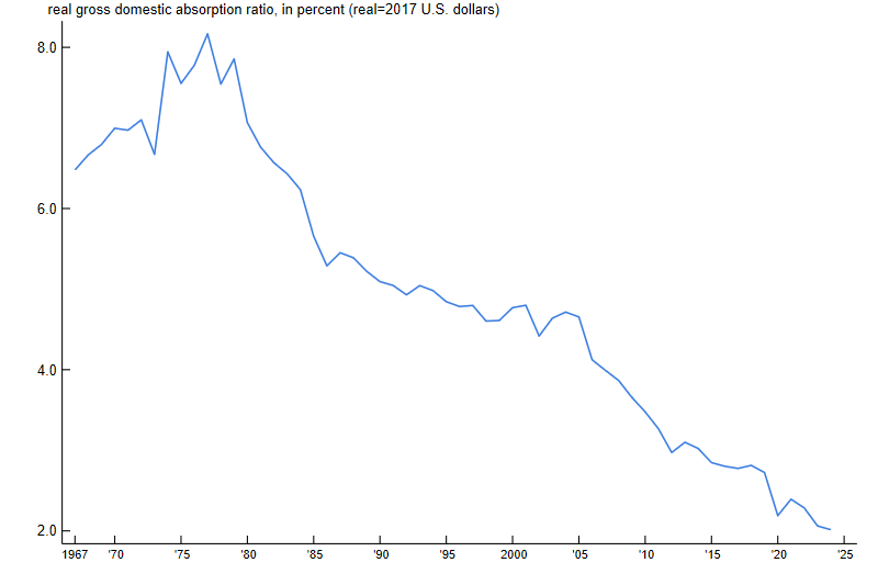
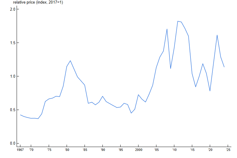
Figure 1 stands in contrast to the common wisdom that the use of oil in the U.S. economy has fallen. In figure 2, we reconcile these two facts. In panel A of figure 2, we plot the real oil share, calculated as the nominal domestic absorption ratio divided by the relative price of petroleum; we compute this relative price as the chain price index for gross output of the petroleum sector divided by the GDP chain price index. As shown in panel A, the real use of oil has indeed steadily fallen relative to real GDP since the 1970s. Panel B of figure 2 shows that the differing trends in the nominal and real absorption ratios are explained by an increase in the price of petroleum relative to the GDP price index. Thus, over the longer run, while the real absorption ratio has trended down, the nominal ratio has moved sideways. As we show next, the nominal ratio is the relevant share for our calculations.
2. The real oil share and the relative price of oil, 1967–2024
A. Real oil share
B. Relative price of oil
Sources: Authors’ calculations based on data from the U.S. Bureau of Economic Analysis, Input-Output Accounts and National Income and Product Accounts of the United States, from Haver Analytics and FRED.
A share-based approach
We apply a share-based approach to assess the potential impact of the recent oil price shock on GDP. Specifically, we apply the results in Baqaee and Farhi (2024), who study an open economy production model with input–output linkages across sectors and countries. They show that in a frictionless economy,3 a second-order approximation yields the impact on real GDP, of a shock to the supply of a sector or factor of production to be as follows:4
where is the nominal share of that factor as a fraction of nominal GDP. In an open economy, the relevant share is precisely the domestic absorption ratio calculated in figure 1: gross output plus imports less exports, which captures total domestic intermediate and final expenditures on that factor, relative to total GDP. By using gross output, the absorption ratio captures exposure both through intermediate and final use of the factor, as well as all network linkages.5 The first term in the expression captures the first-order impact of the shock, which is the direct effect on GDP of a change in the use of the factor holding the absorption ratio fixed; the second term in the expression captures the second-order impact of the shock due to changes in the absorption ratio.6
To implement the calculation, we need to translate the oil price shock into its effect on oil quantities using an estimate of the elasticity of demand for oil. Recent estimates put the short-run elasticity at about –0.1 (when substitution possibilities to alternative inputs are limited, typically thought of as less than one year following the shock) and the longer-run elasticity at about –0.3 (when substitution becomes feasible, typically thought of as more than one year following the shock).7 We use –0.1 for our benchmark scenario and also report results for –0.3 and the lower value of –0.04 preferred by Bachmann et al. (2024). For the purposes of our calculations, we use a 50% increase in the price of oil, which was roughly the rise in the price from just before the conflict through early March (see, e.g., Fisher et al., 2026).8 Multiplying this value by the elasticity of demand yields the implied change in quantity, to use in the equation.
The absorption ratio we use is the average over the period 2015–24 of 2.75%. We calculate the change in the ratio in two ways. First, the change in the ratio can be shown to be related to its level; the elasticity of substitution across inputs, σ (which in a CES environment9 is the negative of the elasticity of demand); and ∆ log
Thus, the change in the ratio can be calculated given an initial ratio and the assumptions in the previous paragraph (which determine σ and Δ log ). In a second approach, we ignore this theoretical connection and simply assume a change in the ratio.
Figure 3 presents the results across five scenarios.
3. The potential impact of the oil price shock on U.S. gross domestic product (GDP)
| Scenario | Price increase (%) | Elasticity of demand | Change in oil quantity (%) | Domestic absorption ratio | Change in domestic absorption ratio | Change in GDP (%) |
|---|---|---|---|---|---|---|
| 1. Low elasticity | 50 | –0.04 | –2.0 | 0.028 | 0.013 | –0.07 |
| 2. Short-run elasticity | 50 | –0.10 | –5.0 | 0.028 | 0.012 | –0.17 |
| 3. Long-run elasticity | 50 | –0.30 | –15.0 | 0.028 | 0.009 | –0.48 |
| 4. Large change in share | 50 | –0.10 | –5.0 | 0.028 | 0.055 | –0.28 |
| 5. Long-run elasticity and large change in share |
50 | –0.30 | –15.0 | 0.028 | 0.055 | –0.83 |
Source: Authors’ calculations.
Our baseline case is scenario 2: A 50% price increase along with an elasticity of demand of –0.1 implies an oil quantity change of –5% and a change in the domestic absorption ratio of 1.2 percentage points. Putting these together yields an impact on GDP of –0.17%. Scenarios 1 and 3 perform the same calculation using lower (–0.04) and higher (–0.3) elasticity values. The results from scenarios 1–3 show that the impact on GDP is increasing with elasticity and ranges from –0.07% to –0.48%.10 Scenarios 4 and 5 ignore the theoretical link between the elasticity of demand and the change in the absorption ratio and assume a large change in the domestic absorption ratio of 5.5 percentage points, which is roughly the change observed across the 1970s. Under this assumption and at the baseline elasticity of –0.1 (scenario 4), the impact on GDP is –0.28%; scenario 5 shows that the impact on GDP can become significantly larger (–0.83%) if both the elasticity is high and the change in the absorption ratio is large. The scenarios in figure 3 thus represent possible bounds on the output effects of the shock, at least as implied by the share-based approach.
Additional effects
The share-based approach used to derive the results in figure 3 assumes frictionless markets and flexible wages and prices. Departures from these assumptions can amplify the output effects of the oil price shock. For example, Blanchard and Galí (2010) develop a simple New Keynesian model with price and wage rigidities where oil enters as an input into both production and final consumption. Their model can yield larger effects of oil price shocks on output, depending on the degree of nominal rigidities in labor and output markets and the monetary policy response to the shock. Larger effects also are present in Fisher et al. (2026), who examine some alternative scenarios for the current oil price shock through the lens of a different medium-scale New Keynesian model.
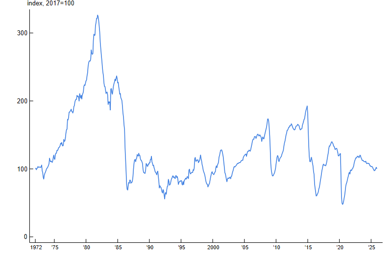
The domestic absorption ratio used for figure 3 treats the domestic and imported oil sectors in the same way and thus may not capture a possible increase in domestic production in response to a spike in global prices. Figure 4 plots real industrial production in oil and gas well drilling and shows that indeed, domestic production may respond to such a shock; e.g., there was a significant increase in domestic production beginning in the late 1970s and into the early 1980s. An expansion in domestic production in response to the recent shock would mitigate the detrimental impact on GDP shown in figure 3.
4. Industrial production: Oil and gas well drilling, 1972–2026
Comparison with the 1970s
As illustrated in figure 1, the gross domestic absorption ratio today is not much different than its level just prior to the oil price shocks of the 1970s. Does that imply that we should expect similar effects in the current episode? The answer is likely no.
First, the size of the shock has been much smaller than in the 1970s. For example, the real oil price increased by over 150% in the second half of 1973 and by about 125% in 1979, according to our calculations using BEA data. Shocks of these magnitudes would lead to much larger impacts on GDP than the 50% shock used in the scenarios presented in figure 3.
Second, the domestic oil and gas extraction sector is more developed today than in the 1970s, and the U.S. became a net exporter of petroleum products in 2020. Thus, reliance on foreign oil has diminished, and the possibility of shortages and rationing is likely lessened.11
Third, as pointed out by Blanchard and Galí (2010), the speed at which wages adjust to changes in economic conditions and the response of monetary policy may have changed in ways that could also mitigate the impact of such shocks.
Notes
1 Specifically, we use The Use of Commodities by Industries tables in the Input-Output Accounts. To calculate the gross domestic absorption ratio, we also use data on U.S. GDP, which we obtain from the BEA’s National Income and Product Accounts of the United States.
2 For example, the share averaged 2.6% over the period 1967–72 and virtually the same over the period 2020–24, according to our calculations using BEA data.
3 By “frictionless,” we mean an economy where markets are perfectly competitive and factors of production are paid the value of their marginal products. (Marginal product is the change in output resulting from employing one additional unit of a specific input while keeping constant all the other inputs.)
4 The method was applied in a similar fashion by Bachmann et al. (2024) and Moll et al. (2023) to study the impact of a decline in energy imports from Russia to Germany following the onset of the Russia–Ukraine war.
5 The absorption ratio is akin to the standard Domar weight in network economies adjusted for imports and exports. In a closed economy, the absorption ratio equals the Domar weight, since gross domestic absorption must equal gross domestic output.
6 In the case of Cobb–Douglas production (and constant consumption shares), the expression is exact and equal only to the first term (first-order effect), since in this case absorption ratios are constant.
7 See, e.g., Caldara et al. (2019). The fact that the nominal oil share today is about the same as in the late 1960s/early 1970s despite significant swings in relative prices suggests that the elasticity may be closer to one (the Cobb–Douglas case) in the very long run.
8 Our calculations assume a one-time permanent change in the oil price. By mid-June 2026, following the announcement of a ceasefire agreement, the oil price has fallen to a level roughly 20% higher than prior to the conflict. Using a 20% rather than 50% price increase yields GDP effects that are roughly 40% of those calculated in figure 3.
9 A CES environment means that firms produce using a constant elasticity of substitution production function, which implies that the elasticity of substitution across factors of production is constant (e.g., it is independent of quantities and prices) and equal to the negative of the elasticity of demand for a factor.
10 Holding the change in the quantity of oil fixed, the impact is decreasing with the elasticity of demand, which is related to substitution possibilities. (See equation 2, noting σ is the negative of the elasticity of demand.) The fact that we find the impact to be increasing with the elasticity of demand stems from the direct effect of the elasticity on our calculation: For a given price shock, a higher elasticity implies a larger change in quantity.
11 In this sense, an apt comparison of the 1970s oil price shocks may be to the semiconductor shortage during the Covid pandemic and its aftermath.