The public pays close attention to Federal Reserve communications about future monetary policy, but it remains an open question how those communications shape the public’s expectations for the path of policy rates. This question is important because such expectations have effects on longer-term interest rates and thereby on the macroeconomy. In this article, we explore how market expectations adjust to the information provided in the “dot plot” of the Summary of Economic Projections (SEP), which contains the Federal Open Market Committee’s (FOMC) assessment of the appropriate future path of the federal funds rate (FFR).¹ The results shed light on the market interpretation of forward guidance and its efficacy as a communication tool.

Using narrow windows around the publication of the FOMC’s SEP over the period 2015–26, we show that financial markets are sensitive to the new information the FOMC participants provide about their expected future paths of policy rates, especially information about how they expect to adjust rates conditional on incoming data, i.e., their “reaction function.” It seems clear, however, that markets do not take FOMC projections at face value because they only adjust partially toward those projections. We estimate that when the dot plot shows a median path of policy rates that is 25 basis points higher than what Fed watchers expected, market pricing initially rises by only 5 basis points. In subsequent quarters, market expectations further adjust toward the initial SEP surprise, while SEP projections are revised somewhat toward the market’s view. The market’s partial adjustment is consistent with the public understanding that SEP dot plots are conditional assessments, not firm commitments, and that considerable uncertainty is embedded in them.

Data

For the SEP, FOMC participants are asked quarterly to report projections of key macroeconomic variables and the FFR at various horizons, assuming appropriate monetary policy. The SEP’s dot plot reports participants’ projections of the FFR for the end of the current year, as well as the next two or three calendar years.²

We measure prerelease expectations for median SEP projections, each quarter, using two separate surveys: 1) the New York Fed’s Survey of Market Expectations (SME),³ which since 2015 has asked market participants about their forecast for the median SEP FFR projections, and 2) a Bloomberg survey that since 2017 has asked for respondents’ expectations for the median SEP projections of FFR, gross domestic product (GDP), inflation, and unemployment.⁴ We compute quarterly surprises by subtracting each survey value from the realized median SEP value at the corresponding projection horizon. The surprises in the median SEP projection of FFR relative to the SME have standard deviations ranging from 12 to 26 basis points across horizons, except for the December SEP projections for the end of the current year (effectively, a two-week-ahead forecast), for which the surprises are always zero.

Our main tests use data at daily and quarterly frequencies. In those specifications, we measure market expectations of the FFR using instantaneous overnight index swap (OIS) forward rates, which allow us to match exactly the horizons of the SEP projections. The forward rates are estimated based on data on OIS rates from Bloomberg.

We also examine high-frequency changes in market expectations around SEP releases, for which we use intraday quotes on other interest rate derivatives, obtained from OneTick. To cover the projection horizons in the SEP, we use FFR futures for the shortest horizon and a combination of Eurodollar (pre-2021) and Secured Overnight Financing Rate (SOFR) (2021–23) futures for the other horizons. We match the maturity of the futures to the SEP horizons as closely as possible. Starting in September 2023, we switch to intraday OIS forward rates at all horizons, as those become available to us and allow us to exactly match the SEP horizons. We lack intraday data for horizons beyond three years.

Market reactions to SEP surprises

In this section, we test how market-based expectations of interest rates react to surprises in the SEP on the days when those surprises occur. We first measure the reactions to surprises in the SEP FFR projections alone, using both daily and intraday data. We then extend the analysis to examine the extent to which these reactions depend on surprises in the SEP macroeconomic projections.

Baseline specification

In our first set of tests, we examine how market expectations for the path of policy rates respond when market participants receive policymaker projections. If the market views the median SEP FFR projections as informative about future policy rates, we would expect market rates to move in the same direction as the surprise; if the market views the projections as strict commitments, we would expect market rates to move one-for-one with the surprise at the corresponding horizon.

Specifically, we run “event study” regressions⁵ of the form $$∆{\mathrm{MKT}}_t^h=\mathrm{\alpha }+{\mathrm{\beta }S\left(\mathrm{ffr}\right)}_t^h+\mathrm{\gamma }({\mathrm{MKT}}_{t-1}^h-{\mathrm{MKT}}_{\mathrm{SMEdate}}^h)+{\mathrm{\epsilon }}_t^h\text{,}$$ where $∆{\mathrm{MKT}}_t^h$ is the change in the market expectation of the policy rate $h$ quarters ahead around the day of the SEP release, $t$; ${S\left(\mathrm{ffr}\right)}_t^h$ is the surprise component of the median SEP projection of the FFR at quarterly horizon $h$; $\mathrm{\alpha }$, $\mathrm{\beta }$, and $\mathrm{\gamma }$ are coefficients to be estimated; and ${\mathrm{\epsilon }}_t^h$ is an error term. The term $({\mathrm{MKT}}_{t-1}^h-{\mathrm{MKT}}_{\mathrm{SMEdate}}^h)$ controls for the update in market expectations between the SME response date (see note 4 for details on the timing of collecting survey responses) and the day before the SEP release. Omitting this term does not have a substantial effect on our results.

We run these regressions both pooling the data across forecast horizons and disaggregating the data by yearly projection horizon—the end of the current year, the next year, and so on. Our baseline specification uses daily changes in OIS forward rates as the dependent variable. We report the intraday results for the sake of robustness, measuring changes in market rates in 30-minute windows around each SEP release. This addresses the concern that the daily changes also embed the information from the post-FOMC-meeting press conference as well as any other news during that day.⁶

As shown in figure 1, the pooled results deliver a coefficient of about 0.2 on the SEP surprise, using either the daily or the intraday data (columns 1 and 2). This coefficient implies, for instance, that when the FOMC surprises the market with a median policy rate projection that is 25 basis points higher than expected, the market adjusts its own forecast by about 5 basis points, on average, on the day of the release. The response is positive and has small standard errors at all horizons (columns 3–8) except the longest one (column 9), where we have fewer observations. Using the intraday data produces coefficient estimates that are similar to those based on daily data, and because the coefficients based on intraday data reflect information in narrower windows, they are more precisely estimated.⁷

1. Reaction of market rates to surprises in the median SEP FFR projections

** Significant at the 5% level.
*** Significant at the 1% level.
Notes: This figure shows the results of regressions (see note 5) of changes in market forward rates on surprises in the Federal Open Market Committee’s (FOMC) median Summary of Economic Projections (SEP) federal funds rate (FFR) projections, relative to the Federal Bank of New York’s Survey of Market Expectations (SME), at matched horizons. The regressions are run on SEP release days using either end-of-day data on overnight index swap (OIS) forward rates or data from a complex of interest rate derivatives in 30-minute windows around the SEP releases. The data are quarterly over the period September 2015–June 2026. Columns 1 and 2 pool all of the data across SEP projection horizons. The remaining columns split the data by the projection horizons. All regressions control for the change in the OIS forward rates that occurs between the SME response date (see note 4 for details on the timing of collecting survey responses) and the day before the SEP release. The standard errors are in parentheses. A definition for adjusted R² is available online.
Sources: Authors’ calculations based on data from the Federal Reserve, Bloomberg, and OneTick.

	Pooled sample			Horizon = End of
				Current year			Next year			Following year			Year after that
	(1) Daily OIS	(2) Intraday		(3) Daily OIS	(4) Intraday		(5) Daily OIS	(6) Intraday		(7) Daily OIS	(8) Intraday		(9) Daily OIS
Median SEP FFR surprise	0.22*** (0.04)	0.20*** (0.02)		0.19*** (0.05)	0.24*** (0.03)		0.34*** (0.09)	0.26*** (0.05)		0.20** (0.08)	0.13*** (0.04)		0.10 (0.13)
Control	Yes	Yes		Yes	Yes		Yes	Yes		Yes	Yes		Yes
Adjusted R²	0.14	0.39		0.35	0.61		0.21	0.47		0.08	0.23		0.01
Number of observations	150	135		43	43		43	43		43	43		21

The fact that the coefficients are substantially less than 1 implies that the projections are initially heavily discounted. A possible interpretation of this partial pass-through is that market participants view the SEP dots as conditional forecasts characterized by substantial uncertainty. The results are broadly consistent with D’Amico and King (2023a), who, using a structural vector autoregression, estimated a similar degree of pass-through from FOMC interest rate signals to survey expectations of the FFR.

One factor that could contribute to uncertainty about the SEP forecast is disagreement among policymakers. We explored this possibility by interacting the median SEP surprises with the interquartile range of policymakers’ FFR projections, but this interactive term explained little and did not substantially change our baseline coefficients. This also suggests that perhaps disagreement among FOMC participants does not diminish the information content of the SEP dot plot. It may also be that the median of the policy rate projections does not fully capture the information that market participants extract from the SEP.

Controlling for surprises in SEP macroeconomic forecasts

If the market views the SEP dot plot as a forecast of the FFR conditional on the macroeconomy, then one might wonder whether the market response reflects a reassessment of the FOMC’s macro outlook or of the FOMC’s reaction to that outlook. To disentangle these two possibilities, we extend the baseline specification in the previous subsection by adding the surprises in the SEP projections of GDP and headline inflation according to the Personal Consumption Expenditures (PCE) Price Index, relative to the Bloomberg survey.⁸ The Bloomberg data begin in 2017 and thus reduce the sample size. Therefore, we focus only on the pooled-horizons specification. Column 1 of figure 2 shows that our baseline coefficient estimate of 0.22 on FFR projection surprises remains nearly the same, at 0.23, in this sample.

2. Reaction of OIS forward rates to surprises in the median SEP FFR and macroeconomic projections

* Significant at the 10% level.
** Significant at the 5% level.
*** Significant at the 1% level.
Notes: This figure shows the results of regressions (see note 5) of changes in overnight index swap (OIS) forward rates on surprises in the Federal Open Market Committee’s (FOMC) median Summary of Economic Projections (SEP) federal funds rate (FFR) projections, relative to the Federal Bank of New York’s Survey of Market Expectations (SME), and in the SEP macroeconomic projections, i.e., projections for gross domestic product (GDP) and headline inflation according to the Personal Consumption Expenditures (PCE) Price Index, relative to the Bloomberg survey, at matched horizons, as discussed in the text. The regressions are run on SEP release days using end-of-day data. Data are quarterly over the period December 2017–June 2026. All regressions control for the change in the OIS forward rates that occurs between the SME response date (see note 4 for details on the timing of collecting survey responses) and the day before the SEP release. The standard errors are in parentheses. A definition for adjusted R² is available online.
Sources: Authors’ calculations based on data from the Federal Reserve and Bloomberg.

	(1) FFR path only	(2) Macro variables only	(3) FFR path and macro variables
Median SEP FFR surprise	0.23*** (0.05)		0.20*** (0.05)
Median SEP GDP surprise		0.06* (0.03)	0.07** (0.03)
Median SEP headline PCE surprise		0.21*** (0.07)	0.13** (0.06)
Control	Yes	Yes	Yes
Adjusted R²	0.15	0.09	0.20
Number of observations	115	115	115

As shown in column 2 of figure 2, the coefficients on the surprises in the SEP projections of GDP and PCE inflation on their own are associated with positive and significant changes in market rates. This is consistent with theory: If the FOMC believes the economy is going to be stronger or inflation higher, the market thinks it is more likely to raise rates in the future. The coefficients are also potentially consistent with the presence of “Fed information effects,” through which the market learns about the future state of the economy from the FOMC’s forecasts.⁹ However, as shown in column 3, controlling for SEP macroeconomic surprises does not considerably change our initial estimate of the effects of the SEP FFR surprise, which remains around 0.2 and precisely estimated.¹⁰

The results in figure 2 suggest that much of the information that the market takes from the SEP is about how the FOMC will behave conditional on the state of the economy, as summarized by the outlooks for GDP growth and PCE inflation. If the market were only learning about future growth and inflation from the SEP, the coefficient on the FFR projections in columns 1 and 3 would be zero. A possible explanation is that it is information about the policy reaction function, rather than forecasts of the economy, that matters most for market expectations.¹¹ Such an interpretation is consistent with Bauer and Swanson (2023) and with Couture’s (2021) finding that the macroeconomic components of the SEP have relatively small effects on asset prices. Still, controlling for the macro surprises does not bring the SEP FFR coefficient anywhere near 1, which continues to suggest that whatever signal the median SEP dot sends about rates is initially discounted by the market.

Reactions over the medium run

We now look beyond the immediate reaction around the SEP projections and analyze how market expectations adjust over time following SEP surprises. We would expect the SEP projection and market forecast for a given date to converge as the date gets nearer, but how quickly this happens and whose forecast is more likely to adjust are empirical questions.

To study this issue, we pool the data and run a vector error-correction model (VECM),¹² modified to account for horizon-varying coefficients. The VECM tells us, at each horizon, how the market and SEP forecasts change, on average, given their past changes and the disagreement between them. By iterating the system forward, we can trace out how the two sets of forecasts evolve as we get closer to a fixed forecast date, starting from a hypothetical initial value.

Specifically, we estimate the model $$∆{\mathrm{SEP}}_t^{h-1}=B_1^h+B_{11}^h∆{\mathrm{SEP}}_{t-1}^h+B_{12}^h∆{\mathrm{MKT}}_{t-1}^h+{\mathrm{\Gamma }}_1^h({\mathrm{SEP}}_{t-1}^h-{\mathrm{MKT}}_{t-1}^h)+e_{1,t}^{h-1}\text{,}$$ $$∆{\mathrm{MKT}}_t^{h-1}=B_2^h+B_{21}^h∆{\mathrm{SEP}}_{t-1}^h+B_{22}^h∆{\mathrm{MKT}}_{t-1}^h+{\mathrm{\Gamma }}_2^h({\mathrm{SEP}}_{t-1}^h-{\mathrm{MKT}}_{t-1}^h)+e_{2,t}^{h-1}\text{,}$$ where we have changed the time convention so that $t$ now indexes quarters (specifically, the time between each SEP release), rather than the daily or intraday changes we used in the event studies estimated in the previous section. Here, we define $∆{\mathrm{SEP}}_t^{h-1}={\mathrm{SEP}}_t^{h-1}-{\mathrm{SEP}}_{t-1}^h$, i.e., the change in the median SEP interest rate forecast for a fixed date, $t+h-1$, between quarters $t-1$ and $t$. Similarly, $∆{\mathrm{MKT}}_t^{h-1}$ is the quarterly change in the OIS forward rate referencing date $t+h-1$. The various $B$ parameters are intercepts and coefficients in these equations, while the $e$’s are unpredictable forecast revisions. Meanwhile, $({\mathrm{SEP}}_{t-1}^h-{\mathrm{MKT}}_{t-1}^h)$ is an “error correction” term, with the coefficients ${\mathrm{\Gamma }}_1^h$ and ${\mathrm{\Gamma }}_2^h$ measuring the amount by which the SEP and the market adjust when their interest rate forecasts differ from each other.

Because there is a strong reason to suspect that rates of convergence in expectations are higher at shorter horizons (e.g., the SEP projection and the market forecast should completely converge between horizons 1 and 0), we let all of the coefficients vary by horizon. Specifically, we allow them to be linear functions of $h$, such as $$B_1^h=a_1+b_{1}h\text{,}$$ where $a_1$ and $b_1$ are parameters to be estimated.¹³

Figure 3 shows the coefficients of the model, reported for ease of exposition at the following horizons: $h$ = 4 quarters (one year) and $h$ = 8 quarters (two years). The coefficients ${\mathrm{\Gamma }}_1$ and ${\mathrm{\Gamma }}_2$ have negative and positive signs, respectively, implying that both the SEP and market projections move toward each other when there is a gap between them. As expected, the magnitude of these effects is somewhat greater, implying faster rates of convergence, at shorter horizons. If markets are efficient, we expect low explanatory power for OIS forward rates, since in principle most predictable variation should be arbitraged away. Consistent with that intuition, the regression for $∆{\mathrm{MKT}}_t^{h-1}$ produces a low $R^2$, meaning that the predictive power of the regression is weak. However, the significant error-correction term does imply that following an SEP surprise, market expectations in subsequent quarters tend to continue to move in the same direction as the surprise. There is also some inertia in the SEP changes, as reflected by the coefficient on its own lag, $B_{11}^h$, although this is not always statistically significant.

3. Selected parameters of VECM

* Significant at the 10% level.
** Significant at the 5% level.
Notes: This figure shows parameter estimates for the horizon-varying vector error-correction model (VECM) described in the text. The parameter values for horizons of four and eight quarters ahead (h = 4 and h = 8) are used for the sake of illustration. The model is estimated on quarterly data over the period September 2015–June 2025, using changes in the Federal Open Market Committee’s (FOMC) median Summary of Economic Projections (SEP) forecasts and overnight index swap (OIS) forward rates at horizons of zero to 13 quarters ahead. A definition for adjusted R² is available online.
Sources: Authors’ calculations based on data from the Federal Reserve and Bloomberg.

Independent variable	Coefficients	h	Dependent variable
			$∆{\mathrm{SEP}}_t^{h-1}$	$∆{\mathrm{MKT}}_t^{h-1}$
$∆{\mathrm{SEP}}_{t-1}^h$	$B_{\mathrm{11}}^h$,$B_{\mathrm{21}}^h$	4 8	0.14 0.26**	0.15 0.23
$∆{\mathrm{MKT}}_{t-1}^h$	$B_{\mathrm{12}}^h$,$B_{\mathrm{22}}^h$	4 8	0.18 0.10	0.06 –0.01
$({\mathrm{SEP}}_{t-1}^h-{\mathrm{MKT}}_{t-1}^h)$	${\mathrm{\Gamma }}_1^h$,${\mathrm{\Gamma }}_2^h$	4 8	–0.10 –0.09*	0.27** 0.13*
Adjusted R² Number of observations			0.21 133	0.02 133

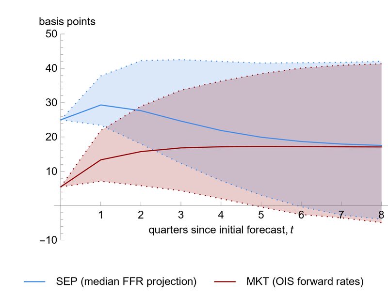
To quantify the market’s overall adjustment to an SEP surprise and illustrate its dynamics, we show in figure 4 the impulse-response function following such a surprise, based on the VECM. For the sake of illustration, we consider an SEP projection surprise at a horizon of eight quarters from when the projection is made, which is roughly in the middle of the set of horizons used in the estimation. Based on the results in figure 1, we assume that when there is a 25 basis point surprise in the SEP at that horizon, the corresponding OIS forward rate moves contemporaneously by 5 basis points in the same direction. That is, starting from the steady state, we consider an initial configuration of $∆{\mathrm{SEP}}_0^8=25$ basis points, $∆{\mathrm{MKT}}_0^8=5$ basis points, and $({\mathrm{SEP}}_0^8-{\mathrm{MKT}}_0^8)=20$ basis points, as shown by the initial values of the impulse responses on the vertical axis of figure 4.

4. Dynamic responses to a 25 basis point surprise in the median SEP FFR projections eight quarters in advance

Based on the median estimates, after the initial shock, the SEP FFR projection moves up somewhat further because of the positive value of $B_{11}$, but eventually it settles at a realized interest rate about 18 basis points above its pre-shock value. Meanwhile, over about two quarters following the SEP surprise, the market expectation (as captured by OIS forward rates) moves up to the same 18 basis point level, reflecting the effects of both $B_{21}$ and ${\mathrm{\Gamma }}_2$. Neither the SEP nor the market reaction is consistent with fully rational expectations, since the SEP forecasts initially overshoot the eventual adjustment in the FFR, while the OIS forward rates are slow to catch up.¹⁴ However, the statistical uncertainty around these responses is fairly high, and the responses of the SEP and the market are statistically indistinguishable after about two quarters. The fact that the realized FFR does ultimately turn out to be higher than initially projected following a positive SEP surprise—albeit with weak statistical significance—implies that the SEP is indeed informative about the future course of the FFR, even eight quarters in advance.

Conclusion

The results in this article shed light on the role that the FOMC’s SEP projections play in shaping expectations about monetary policy. The market clearly pays attention to the information contained in the SEP dot plot and adjusts its forecasts of policy rates in response. We would expect the market to do so because, as shown in figure 4, SEP projections are informative about future interest rates. These findings, together with those in figure 2, suggest that the SEP FFR projections allow the public to learn something about the FOMC’s reaction function earlier than it otherwise would. The early revelation of this information should allow agents to make decisions in advance of actual changes in the FFR, accelerating the transmission of monetary policy. However, we also find that the market only partially and gradually takes on board the unexpected changes in the SEP projections. That result is consistent with the market understanding the SEP dot plot to be an uncertain conditional forecast, rather than a firm commitment, and discounting it accordingly.

Details for Thomas B. King are available on his Federal Reserve Bank of Chicago online profile (accessed by clicking his name in the byline). Stefania D’Amico is a policy and research advisor to the System Open Market Account manager at the Federal Reserve Bank of New York. Francisco Torralba is a financial modeling and quantitative analytics principal in the Markets Group at the Federal Reserve Bank of New York. The New York Fed staff report version of this research (D’Amico et al., 2026) was published concurrently.

---

Notes

¹ The FFR is the FOMC's main policy tool. It is the interest rate at which depository institutions lend reserve balances to other depository institutions overnight. Changes in the FFR trigger changes in other short- and medium-term interest rates, the foreign exchange value of the U.S. dollar, and other asset prices that influence households’ and businesses’ spending and investment decisions. The dot plot was introduced in the SEP in January 2012, as shown in this timeline of the SEP and other Federal Reserve communications.

² In March and June, the SEP includes three forecast horizons, and in September and December, it includes four.

³ The SME is the result of the consolidation, in January 2025, of two New York Fed surveys, the Survey of Primary Dealers and the Survey of Market Participants. Prior to 2025, we pool the responses from the earlier two surveys.

⁴ Before January 2025, the two New York Fed surveys that were consolidated as the SME (see note 3) did not ask about expectations for SEP projections of macroeconomic variables. The SME polls financial firms that are market participants, whereas the Bloomberg survey includes some firms that are not market participants. For our sample, we use both surveys, whose sample sizes are 50–70 firms. The two surveys differ in their collection periods by about three days, with the SME responses being collected about nine days before the SEP release and the Bloomberg survey responses about six days before.

⁵ A regression is a statistical process that measures the degree of correlation between two variables—an independent (predictor) variable and a dependent (response) variable—while holding constant the other independent variables; the estimated coefficient from a regression represents the mean change in the dependent variable for a one-unit change in the independent variable.

⁶ Note that the 30-minute window includes the market reaction to the combination of news contained in the SEP and FOMC statement following the FOMC meeting, since they are released at the same time. If the statement carried news that was systematically correlated with the news in the SEP, our estimated coefficient would capture the effects of both. Martinez and Sinclair (2026) show that a sizable share of the monetary policy surprises in Bauer and Swanson (2023) is explained by SEP surprises filtered through the Taylor rule.

⁷ We also ran these regressions after orthogonalizing the SEP surprises with respect to the moves in OIS forward rates that occur from the prior SEP to the SME response date. (In this context, orthogonalizing means adjusting explanatory independent variables so that they are not correlated with one another.) In that case, the estimated coefficients in the intraday regressions fall a bit, but the daily coefficients are essentially unchanged.

⁸ We also ran versions of this regression using surprises in the SEP projections of unemployment and core PCE inflation (which removes the more volatile food and energy components), but those surprises had less explanatory power.

⁹ See, among others, Campbell et al. (2012) and Nakamura and Steinsson (2018).

¹⁰ Orthogonalizing the FFR surprise with respect to the macro surprises does not change the size and significance of the coefficient.

¹¹ Our estimate of the market’s reaction to FFR projections could also be driven by surprises in aspects of policymakers’ macroeconomic assessments that surveys do not capture, such as uncertainty about their forecasts.

¹² An introduction to VECMs is available online.

¹³ This is equivalent to including terms that interact the intercept and each of the three variables in the model with $h$. We also ran a standard VECM specification restricting all of the coefficients to be the same across horizons. In that model, the results were similar, though convergence was a bit slower.

¹⁴ Engstrom (2026) also finds that market expectations are slow at incorporating new information and attributes this in part to the anchoring effect of the SEP dot plot. However, we find that the market expectations adjust slowly also to the SEP dot plot as the market partially discounts the SEP signal.

---

Opinions expressed in this article are those of the author(s) and do not necessarily reflect the views of the Federal Reserve Bank of Chicago or the Federal Reserve System.