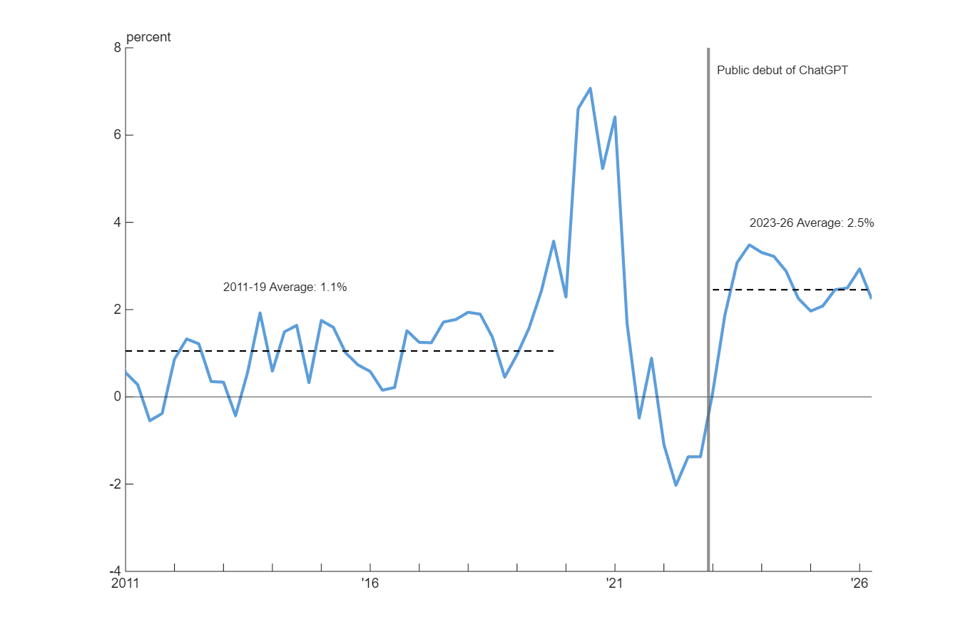
Computer scientists and business leaders have been touting the productivity-enhancing benefits from applications of artificial intelligence (AI) and related technology that they think are starting to materialize and expect to see in the future. Economists and the public seem to have adopted this view as well.1 Figure 1 shows that following the wild swings of the pandemic period, nonfarm private business labor productivity growth (total output divided by total hours worked in the sector) has indeed accelerated. It has been growing by about 2.5% per year compared with the pre-pandemic average of 1.1%. Perhaps coincidently, the faster productivity growth began soon after the public debut of ChatGPT in late 2022. Productivity growth is a key metric for monetary policymakers as it influences the rate of interest that keeps savings and investment in balance, the so-called natural rate of interest, otherwise known as r*.
1. Nonfarm private business labor productivity growth in the United States, 2011–26
Source: Authors’ calculations based on data from the U.S. Bureau of Labor Statistics, Office of Productivity and Technology, from FRED.
On May 8, 2026, Chicago Fed President Austan Goolsbee discussed the implications of faster productivity growth for monetary policy at a conference hosted by the Hoover Institution at Stanford University. He argued that if the central bank sets the interest rate using a version of the Taylor (1993) rule that tracks the natural rate of interest, the implications for rate setting depend on whether the increase in productivity growth is anticipated or not.2
Goolsbee argued that expectations that productivity growth will be faster in the future create an incentive to pull forward consumption spending before the higher levels of productivity have been realized. For example, the anticipated productivity growth should be capitalized in stock prices and make households feel richer and want to consume more. In this case, the natural rate of interest rises to discourage consumption and close the gap between desired consumption and output. When the Taylor rule tracks the natural rate, this leads to a higher policy rate (and thus a higher nominal interest rate). If productivity growth is unanticipated, there is no incentive to pull consumption forward and the natural rate is unaffected. Just as when such growth is anticipated, the realized productivity growth lowers costs and inflation. Since the Taylor rule depends on the gap between actual inflation and the central bank’s inflation target, the lower inflation dictates a lower policy rate.
In this Chicago Fed Letter, we elaborate on the arguments in Goolsbee’s speech, provide some of the details behind the simulations he reported, and describe the results of some robustness exercises suggested by Federal Reserve Governor Chris Waller at the Hoover Conference.
The model
We work with a simple New Keynesian general equilibrium model.3 The model consists of households, firms, and a central bank with a dual mandate of stable prices and maximum employment (like the Federal Reserve’s). Households supply labor to the firms and consume their output. Firms produce output with a simple production function equal to labor productivity multiplied by the quantity of labor input. Wages and prices are sticky, meaning they are slow to adjust to shocks. There is no capital, but the qualitative results are robust to adding it. In this simplified economy without capital, there is also no capital investment; thus savings in physical capital, which equal investment in equilibrium, must be zero. Households can in principle borrow and save using risk-free bonds with the interest rate set by the central bank. We assume these bonds are in zero net supply. Therefore, the interest rate needs to adjust in such a way that there is no savings in bonds or physical capital in equilibrium.4
Monetary policy is set according to a version of the Taylor (1993) rule that tracks the natural rate of interest. In the original Taylor rule the policy rate is set equal to a constant natural rate plus the contributions of the gap between inflation and the central bank’s inflation target (which supports stable prices, one of the pillars of its dual mandate) and the gap between actual output and the level of output consistent with price stability (otherwise known as potential output). The output gap stands in for the other pillar of the central bank’s dual mandate, maximum employment. In practice the natural rate changes over time.5 We replace the constant in the Taylor rule with the model’s time-varying natural rate, which is calculated as the interest rate in the version of the model without sticky wages and prices. A Taylor rule that tracks the natural rate is optimal in many New Keynesian models.6
We now consider several scenarios beginning from the model’s steady state to illustrate the importance of anticipated versus unanticipated productivity growth for determining interest rates.
Monetary policy with unanticipated productivity growth
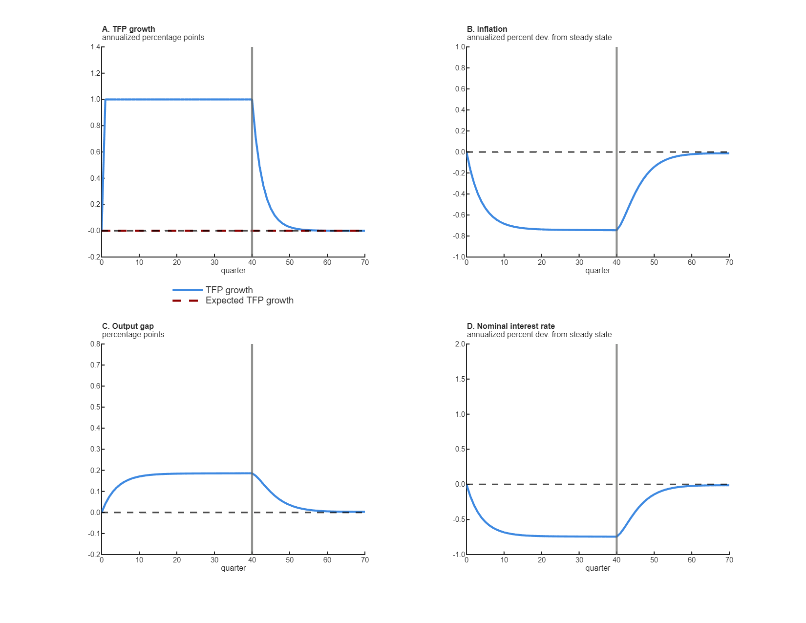
Figure 2 shows simulations with an increase in total factor productivity (TFP)7 of 1 percentage point per year above the model’s steady state. Importantly, the entire productivity growth surge here is a surprise; i.e., each period agents expect productivity growth to return to steady state in the next period. Panel A shows the actual productivity growth as a solid blue line and what people expect each year as a dashed red line. Since agents always expect steady-state productivity growth, the natural rate of interest stays at its steady-state level.
2. Ten-year increase in productivity growth with agents repeatedly surprised
Source: Authors’ calculations.
As one would expect from a productivity surge, inflation falls (see panel B of figure 2). With stickiness, wages are slow to catch up with the higher productivity, so marginal costs fall and production ramps up. The productivity surge raises output higher than its potential and generates a positive output gap (panel C). But you can see in panel D that the low inflation more than offsets the increase in the output gap so that the Taylor rule calls for lowering the nominal interest rate. The model suggests that a 1 percentage point increase in annualized productivity growth should lead to an interest rate cut of about 75 basis points through the duration of the surge.
In his Hoover remarks in May 2026, Goolsbee compared this scenario to the productivity growth acceleration in the mid-1990s. The acceleration was not clear in real time as it had yet to show up in the data. Fed Chairman Alan Greenspan argued back then that because there were strong corporate profits, declining unemployment, rising wages, and falling inflation, it must mean productivity is growing faster, and on that basis, he argued against raising rates.
Monetary policy with anticipated productivity surges
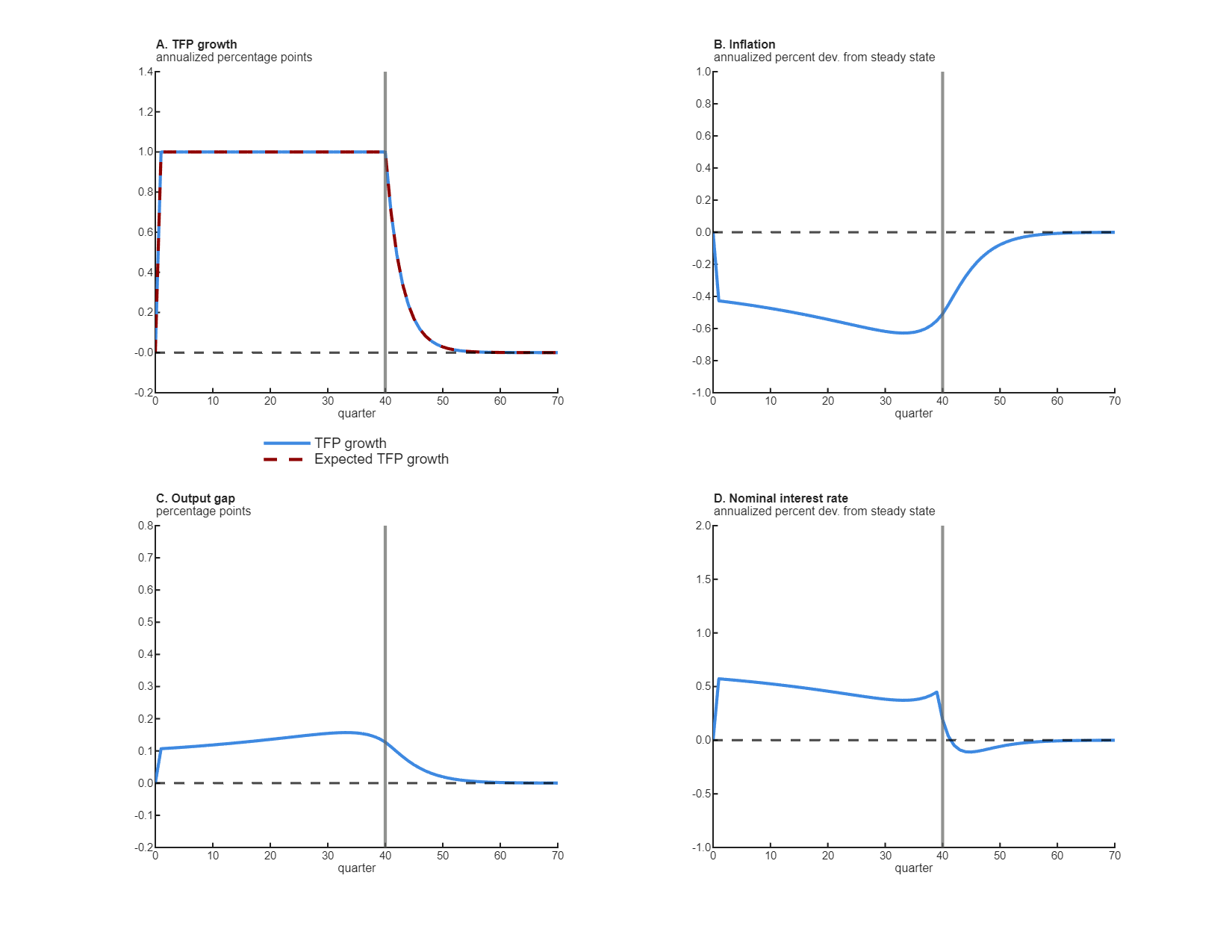
Figure 3 illustrates an identical ten-year surge in total factor productivity, but this time under the assumption that people fully expect it. The solid blue line (actual productivity) and the dashed red line (anticipated productivity) in panel A are the same. When everyone knows that faster productivity growth is coming, inflation still falls about as much as it did when the faster growth is unanticipated (see panel A of figure 2). Firms lower prices from the outset (or raise them by less) because they anticipate lower costs and because their price will be sticky when the higher productivity is realized. Output also heats up just about the same, but something very different happens with the interest rate. The nominal rate does not fall. Instead, it rises.
3. Ten-year increase in productivity growth with perfect foresight
Source: Authors’ calculations.
Since everyone knows there will be extra productivity growth coming, consumers’ anticipated lifetime income is higher, so they try to raise their consumption now. But most of the productivity growth is still on the way—capacity has not expanded yet. Shifting from the future to spend now threatens to overheat the current economy, so the central bank needs to raise the return on savings and get people to reduce spending. If it does not, the economy will overheat today and inflation will rise. The natural rate of interest rises because of the anticipated consumption growth, and the Taylor rule says the central bank must raise the nominal interest rate. Fully anticipated productivity growth of 1 percentage point per year over ten years leads to an interest rate increase of about 50 basis points for the length of the surge.
In his Hoover speech this past May, Goolsbee drew an analogy to the late 1990s. By then productivity data had confirmed Greenspan’s mid-1990s conjecture about productivity growth, and Goolsbee argued that if people expected a rise in structural productivity, even if this growth was not later realized, they would have pulled forward aggregate demand before the gains arrived. In response to the inflationary pressures this would create, monetary policy would have naturally tightened. Consistent with this, the Federal Reserve raised rates six times in less than a year in 1999–2000.
The cost of waiting
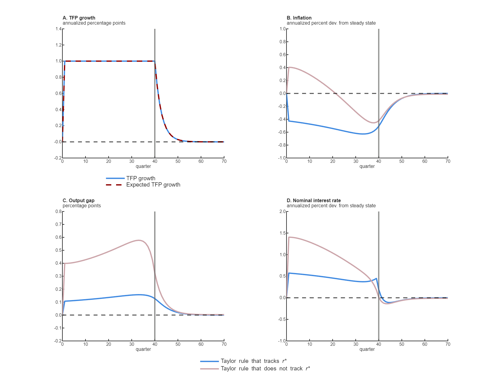
In the case where productivity growth is fully expected, if the central bank decided not to track r* and instead waited until there are actual inflation and overheating before acting, then the inflation picture would be quite different. Take the same simulation as before with a fully expected ten-year productivity surge, but now assume that the central bank does not pay attention to the way productivity growth influences r* and leaves it unchanged in its Taylor rule. In this case the central bank does not offset the wealth effect of higher expected productivity. It only responds once it sees the inflation and output gaps open up.
The results are shown in figure 4. Panel A is just reproduced from figure 3, as are the blue lines in panels B, C, and D—which represent the scenario when the central bank adjusts its policy to account for the change in r*. The pink lines in panels B, C, and D correspond to the scenario in which the central bank adopts a reactive approach that does not consider r*. We refer to this as a “wait-for-it” policy approach because the central bank changes nominal rates only when changes to inflation or the output gap occur. You can see that the wait-for-it strategy generates much higher inflation and a much more overheated economy than when the central bank considers the impact of higher productivity growth on r*. In the end, the central bank has to raise nominal interest rates by more than if it had tracked the natural rate of interest from the beginning.
4. Ten-year increase in productivity growth with perfect foresight: Implications of tracking r*
Source: Authors’ calculations.
Robustness
After Chicago Fed President Austan Goolsbee gave his remarks at the Hoover Institution this past May, his co-panelist Federal Reserve Governor Chris Waller suggested that the wealth effects were relatively small in practice and that the simulation results might not be robust to modifications that would dampen these effects.8
First, Waller argued that the results might weaken if agents exhibited habit persistence in consumption, in which case they would have a strong incentive to keep consumption from changing very much from period to period and might not try to pull consumption forward when productivity growth is anticipated to increase. We have extended the model to allow for empirically plausible habit persistence (the habit parameter is assumed to equal 0.7, which falls within the range of estimates in the macroeconomics literature). Although the habit parameter does result in smoother consumption responses to the TFP shock, our qualitative findings do not change significantly.9
Second, Waller suggested introducing so-called hand-to-mouth consumers that do not have the ability to pull consumption from the future by borrowing. At the extreme of all households being hand-to-mouth, r* would not change because it is not possible to pull consumption forward. More realistic calibrations suggest that roughly one-third of consumers are hand-to-mouth. When we modified our model to incorporate about one-third hand-to-mouth consumers, our qualitative findings survived.10 Intuitively, since hand-to-mouth households cannot save by assumption, the natural rate of interest is determined by those who in principle can. It is enough to have a fraction of agents who want to save and adjust their consumption growth accordingly to have implications for the natural rate.11 The results are also robust if we combine habit persistence with hand-to-mouth consumers.
Conclusion
Productivity growth is a clear winner for the economy as a whole. What it means for interest rates, though, is more subtle. We have used an off-the-shelf simple New Keynesian model to show it depends very much on whether the productivity growth is expected to come in the future or arrives unexpectedly. If it happens unexpectedly, a central banker following the Taylor rule that tracks the natural rate of interest should probably lower nominal interest rates. But the more that productivity growth is expected to come in the future, the more it induces shifting economic activity from the future to the present—and the more necessary it might be to drive up interest rates now to prevent an overheating economy.
1 Indeed, Ezra Karger from the Chicago Fed led a survey of economists, people in the technology sector, and the public about the future implications of AI and found that the median person in each group expects a significant boost to annual productivity growth coming in the next ten years (Karger et al., 2026). The Organisation for Economic Co-operation and Development (OECD) (Lane et al., 2023) and McKinsey & Company (Tinkoff et al., 2026) reach similar conclusions.
2 A brief primer on the Taylor rule, as well as other policy rules, is available online.
3 See the technical appendix for a detailed description of the model we study, the parameter values we use, and more information on the robustness exercises discussed in the penultimate section of this article.
4 The zero net supply assumption is for convenience only. Suppose risk-free government bonds are in positive net supply. In this case, without physical capital, in equilibrium savings would equal the stock of outstanding debt. The interest rate and consumption would be the same as in the economy with bonds in zero net supply.
5 See, e.g., Laubach and Williams (2003), Del Negro et al. (2017), and Bernanke (2005)
6 See, e.g., Barsky et al. (2014); notably, Gilchrist and Leahy (2002) were among the first to make this point.
7 According to the U.S. Bureau of Labor Statistics (BLS), “TFP measures the efficiency of labor, capital, and other countable inputs” of an economy (or a sector, firm, etc.), and “TFP tells us how much can be produced without adding more inputs.” Labor productivity measures the efficiency of labor inputs. In our model without capital, labor productivity is equivalent to TFP.
8 See Waller’s feedback following Goolsbee’s speech starting at the 48:20 mark in the video playback available online.
9 See subsection 8.1 of the technical appendix.
10 See subsection 8.2 of the technical appendix.
11 Kaplan et al. (2014) study “wealthy” hand-to-mouth households. These are households that have a lot of their wealth in illiquid form (e.g., a house or college tuition fund), so that in practice they act like they are hand-to-mouth. Extending the model to include this type of household would effectively raise the share of hand-to-mouth consumers and could possibly overturn our findings. However, in our model the results are robust to raising the share of hand-to-mouth consumers to 99%. (The interest rate is irrelevant when all consumers are hand-to-mouth.)