


The Covid-19 pandemic imposed severe fiscal strain on state and local governments across the United States. Public sector revenues collapsed as economic activity ground to a halt. At the same time, demand for public services surged. To prevent a fiscal contraction that would deepen and prolong the economic downturn, Congress passed the American Rescue Plan Act (ARPA) in March 2021. ARPA authorized nearly $2 trillion in relief across multiple programs, with $350 billion set aside specifically for subnational governments through the State and Local Fiscal Recovery Funds (SLFRF) program. This made SLFRF allocations one of the largest direct intergovernmental fiscal transfers in U.S. history. In this Chicago Fed Letter, we explore how this program impacted local economies. We first estimate the impact of the spending increase on state-level nonfarm employment. We then explore how states chose to spend their funds across different categories of spending and whether some projects were more effective than others at fostering employment.
SLFRF funds made up a large share of state expenditure
The State and Local Fiscal Recovery Funds program allocated money to state, local, tribal, and territorial governments using a series of formulas tailored to each tier of government. State governments received a base allocation of $500 million plus an additional amount proportional to the state’s share of the nation’s unemployed workers during October–December 2020. The added amount was designed to explicitly direct resources to states that experienced greater labor market disruption from the Covid-19 pandemic. County governments were allocated an amount proportional to their 2019 population, while smaller local governments—i.e., those with populations below 50,000—were allocated funds according to their most recent annual operating budget. Finally, metropolitan areas received an additional amount based on a formula that incorporated multiple indicators of local economic conditions.1
SLFRF recipients were permitted to direct their funds to a number of uses. The three main spending categories were as follows: 1) responding to the public health emergency and its economic impacts, including assistance to households, small businesses, and nonprofits; 2) investing in infrastructure, particularly water, sewer, and broadband systems; and 3) replacing lost public sector revenue to maintain government services, encompassing in practice a wide range of needs, including hiring public sector employees. In 2022, an update to the policy expanded the acceptable projects classified under the second and third spending categories (U.S. Department of the Treasury, 2022).
The U.S. Department of the Treasury tracked SLFRF spending through quarterly project-level reports covering the period between March 2021 and March 2026. For our analysis we focus on the reports covering the period between March 2021 and December 2025.2 Each report recorded the government recipient, project type, amount obligated (i.e., formally earmarked for a specific use), and amount expended. By December 2024, 99% of all SLFRF funds had been obligated, while 75% of those obligated funds had been spent, according to our calculations using data from these reports. For the purpose of our analysis, we aggregate all funds to the state level. That is, we add up the funds received by the state and all its counties and local governments to obtain a state-level measure of the total SLFRF allocation.
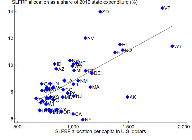
Figure 1 summarizes the size of the SLFRF program by state. It shows the per capita SLFRF allocation to each state (according to the state’s total allocation and its 2019 population) on the horizontal axis, which ranged from $670 in Florida to $1,900 in Wyoming, and the SLFRF allocation as a share of total state expenditure in 2019 on the vertical axis, which ranged from about 6% to 14%.
1. SLFRF allocation as a share of 2019 state expenditure and per capita based on 2019 population
Sources: Authors’ calculations based on data from the U.S. Department of the Treasury, State and Local Fiscal Recovery Funds program; and U.S. Census Bureau, Census of Governments, Annual Survey of State and Local Government Finances, and population statistics.
While the two measures of the size of the program reported in figure 1 are positively correlated, they are not identical because the baseline level of expenditure per capita varies across states. For the sake of consistency with the previous literature, our analysis focuses on the SLFRF allocation as a share of 2019 state expenditure (i.e., the vertical axis in figure 1). Our empirical analysis exploits the variation of the size of the SLFRF program across states to estimate its impact on employment—namely, low-expenditure states generally received a larger amount of funds. If, after controlling for potential confounding factors, we find that those states also saw higher growth in employment from 2022 onward, we obtain a measure of the employment impact of the SLFRF allocation.
Using the allocation size to estimate the impact of SLFRF on employment
An extensive literature studies the impact of public spending on local economic outcomes and generally finds mixed results depending on a variety of factors, such as public spending type, the level of economic slack at the time of expenditure, and econometric specification (Bom and Ligthart, 2014; Ramey, 2021; and Pinto and Waddell, 2025). Most closely related to our analysis, Wilson (2012) exploits cross-state variation in federal transfers from the American Recovery and Reinvestment Act (ARRA) to study its effect on employment. He finds that ARRA created or saved around eight jobs per one million dollars spent. Given the large magnitude of the SLFRF funds relative to states’ existing spending, along with the limited restrictions on how states could choose to use the funds, we are interested in the extent of the SLFRF’s impact on a state’s nonfarm employment level.
Our definition of the budget increase to a given state is its SLFRF allocation relative to its pre-pandemic expenditure (the vertical axis in figure 1):
1) .
Following Jordà (2005), we estimate the magnitude and timing of the effect of SLFRF allocations on total state nonfarm employment.3 Fixing t = 2021, we estimate the following:
2) ,
where is log level of nonfarm employment years in the future (=0,…,3) in state , is the budget increase defined in equation 1, is the -year lag of nonfarm employment (=1,…,4), and is a set of controls, including the state’s unemployment level relative to the national level in the fourth quarter of 2020, the total non-SLFRF pandemic aid as of 2020, and Covid-19 deaths per capita in 2020.4
The results from estimating this regression (equation 2) are found in figure 2. The point estimates suggest that a 1 percentage point increase in a state’s SLFRF allocation (relative to its 2019 budget) resulted in a 0.26% increase in employment in 2022 and around a 0.18% increase in employment in 2023, although the latter estimate is not statistically different from zero. Similarly, the effect is positive, but not statistically different from zero, in 2024. The SLFRF funds amount to about 9% of total state spending on average (see figure 1); therefore, the estimates in figure 2 suggest that SLFRF allocations increased employment by about 1.6%–2.3% nationally in 2022 and 2023.5
2. Impact of the SLFRF allocation on total nonfarm employment
| Log nonfarm employment | ||||
|---|---|---|---|---|
| 2021 | 2022 | 2023 | 2024 | |
| Budget increase coefficient | 0.00124 | 0.00258* | 0.00182 | 0.000514 |
| (0.00114) | (0.00147) | (0.00193) | (0.00231) | |
| Number of observations | 50 | 50 | 50 | 50 |
Because there were 152.6 million jobs in the nonfarm sector in 2022 based on data from the U.S. Bureau of Labor Statistics (BLS), the estimates in figure 2 suggest that the SLFRF increased employment by about 3.6 million jobs up to that year, according to our analysis. As the total cost of the program was $350 billion, we estimate that this amounts to an implied cost of approximately $97,000 per job. This is within the range of values estimated in the literature for other government programs, as summarized in figure 3.
3. Estimated cost per job created or saved by government spending in the literature
| Study | Program | Cost per job |
|---|---|---|
| Chodorow-Reich et al. (2012) | ARRA Medicaid | $26,300 |
| Suárez Serrato and Wingender (2016) | Federal transfers | $30,000 |
| This research | SLFRF | $97,000 |
| Wilson (2012) | ARRA | $125,000 |
| Conley and Dupor (2013) | ARRA highways | $200,000 |
Significant variation in states’ spending on infrastructure
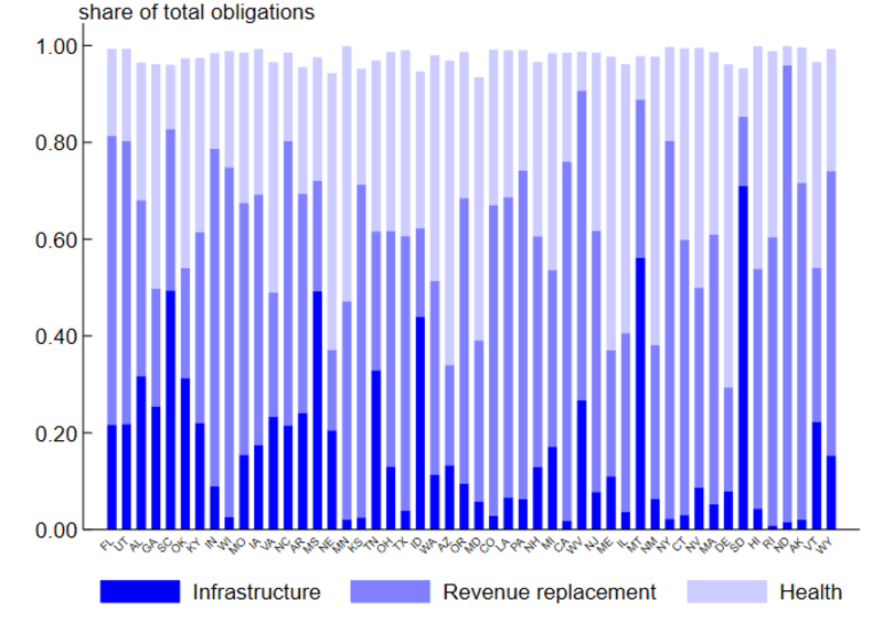
Different forms of public spending may have different employment effects. We exploit the different ways that states chose to use their allocated SLFRF funds to assess whether specific spending categories led to larger changes in employment. Figure 4 shows that the shares of obligated SLFRF funds (up through 2024) across the three largest spending categories—infrastructure, health, and revenue replacement—vary significantly across states. We focus on infrastructure spending, which is often used by government to stimulate the economy in recessions and has been documented in the literature to have significant employment or output effects; see Leduc and Wilson (2014) for an overview of the relevant literature.
4. Share of cumulative obligations of SLFRF funds (up through 2024) in the main expenditure categories
Source: Authors’ calculations based on data from the U.S. Department of the Treasury, State and Local Fiscal Recovery Funds program.
A challenge with using this source of variation to understand the effect of different spending types, however, is that states’ spending choices across categories are not random. For example, suppose that states that were more adversely affected by the Covid-19 pandemic were more likely to spend their allocated funds on infrastructure projects to jumpstart their local economies. If that were the case, their employment growth would appear to be slower because of lingering pandemic effects, rather than because they spent a larger share of the funds on infrastructure. Conversely, if the worst affected states were more likely to spend on health (because they had more sick people from Covid-19) or on revenue replacement (because they had bigger drops in tax collections), our estimate of the impact of the SLFRF program on employment would be biased in the opposite direction. We find negative correlations when we plot both of the following based on 2019 state populations: 1) per capita health spending obligated through December 2024 against per capita Covid-related deaths in 2020 and 2) per capita infrastructure spending obligated through December 2024 against unemployment growth between January and June 2020 (not shown).6 These correlations (using pre-ARPA data on Covid-related deaths and unemployment growth) imply that a standard regression coefficient could potentially be biased upward as states with better outcomes (i.e., fewer deaths or lower unemployment growth) also spent more money per capita on health and infrastructure. This motivates both our use of an instrument, which we explain in the next section, and our inclusion of Covid deaths and unemployment growth as controls in our regressions presented in later sections.
Using the stock of debt to identify a causal effect of infrastructure spending on employment
To address the fact that places that choose to spend on infrastructure may have systematically different post-2020 employment trajectories than places that choose other forms of expenditure, we use an instrumental variables (IV) approach. Economists often try to identify a variable called an instrument that predicts variation on the treatment (in this case share of infrastructure expenditures) but does not otherwise have a direct effect on the outcome (in this case employment). Then, seeing how the outcome responds to the instrument can be regarded as a “natural experiment” that more accurately shows the causal effect of the treatment on the outcome. In our case, a valid instrument must therefore affect the extent to which a state chooses to spend its SLFRF allocation on infrastructure projects (rather than on revenue replacement or health); however, it should not directly affect the state’s level of employment other than through the infrastructure spending channel.
A natural candidate for an instrument in our IV exercise is the state’s pre-pandemic budget situation, captured by its level of 2019 debt per capita. This is a valid instrument if the following two conditions are satisfied: 1) the pre-pandemic level of debt per capita meaningfully impacts the state’s propensity to spend its SLFRF funds on infrastructure projects; and 2) controlling for other variables in the analysis (including the pre-pandemic level of employment), the accumulated stock of debt of a state prior to the pandemic does not directly impact its employment from 2021 onward. In other words, the only way debt per capita impacts future employment must be through how it changes the state’s allocation of SLFRF funds across spending categories.
This second condition cannot be directly tested empirically and is therefore our main assumption. The economics literature has not found a meaningful relationship between debt and future growth prospects across countries (Panizza and Presbitero, 2013), which suggests there may be no direct effect of a state’s debt on its future employment. If the large stock of debt that a given state inherited in 2019 was due, say, to a one-time exceptional event in the past (e.g., an extreme weather event), there should be no reason to expect a correlation with its post-pandemic employment levels. If instead the large stock of debt was due to, say, poor choices in the stewardship of funds—and if this is a characteristic of state governments that persists over time—then it would be conceivable that states with high debt in 2019 would experience smaller employment growth from then on, independently of how they allocated their SLFRF funds. Another potential issue that could threaten the validity of our approach is if a lot of state debt is due to previous infrastructure spending; if high-debt states already have a lot of infrastructure and wouldn’t need more, then the instrument would have a direct impact on the propensity to spend SLFRF funds on infrastructure. To make such scenarios less likely, our regression controls for several variables that we detail in the two subsequent sections, including a measure of past infrastructure spending.
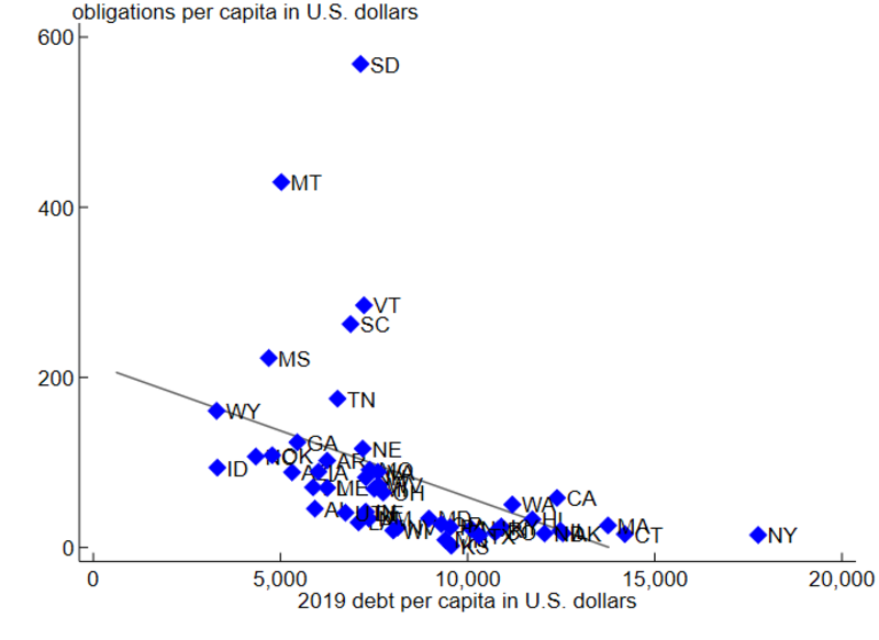
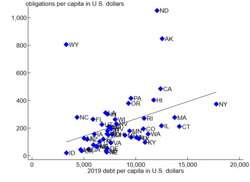
In contrast to the assumption that there is only an effect of debt on employment through infrastructure spending, we can test the first condition for a valid instrument empirically—namely, we can verify that the pre-pandemic budget situation has a statistically meaningful relationship with how a state spends its SLFRF funds. Figure 5, panel A shows the relationship between 2019 debt per capita and total infrastructure obligations of SLFRF funds (in U.S. dollars per capita in 2019) as of December 2024. Figure 5, panel B shows a similar graph for revenue replacement. We find that states with higher pre-pandemic debt obligations were less likely to use SLFRF money toward infrastructure projects and correspondingly more likely to spend it toward revenue replacement; by contrast, health spending (not plotted in figure 5) shows no correlation with pre-pandemic debt per capita. That is, we find the first condition required for the validity of our instrument holds.
5. Cumulative infrastructure and revenue replacement obligations of SLFRF funds (up through 2024) per capita in 2019 versus 2019 debt per capita
A. Cumulative infrastructure obligations versus 2019 debt per capita
B. Cumulative revenue replacement obligations versus 2019 debt per capita
Sources: Authors’ calculations based on data from the U.S. Department of the Treasury, State and Local Fiscal Recovery Funds program; and U.S. Census Bureau, Census of Governments, Annual Survey of State and Local Government Finances, and population statistics.
First-stage estimation
To test this “first-stage” relationship formally, we estimate the following equation, fixing t=2023:
3) ,
where is state ’s per capita amount obligated to infrastructure (or, alternatively, the infrastructure obligations as a share of the state’s 2019 infrastructure expenditure) and is its 2019 debt per capita. We additionally control for four lags of employment and state gross domestic product (GDP), as well as a host of variables described in the next section, which covers the second-stage equation (they’re also listed in the notes under the results reported in figure 6).
The results of the first stage of our IV analysis are found in figure 6.7 We find that 2019 debt per capita is statistically significant in predicting cumulative infrastructure obligations, but not cumulative revenue replacement or health obligations, of SLFRF funds in 2023. An additional $100 of debt per person decreases spending on infrastructure by $1.70 per capita and on health by $0.93 per capita, but increases spending on revenue replacement by $2.46 per capita.
6. First-stage results: Obligations of SLFRF funds in main expenditure categories
| 2023 cumulative infrastructure obligations per capita | 2023 share of infrastructure obligations in total infrastructure expenditure | 2023 cumulative revenue replacement obligations per capita | 2023 cumulative health obligations per capita | |
|---|---|---|---|---|
| 2019 debt per capita | –0.0170*** | –0.00144*** | 0.0246 | –0.00926 |
| (0.00569) | (0.000546) | (0.0197) | (0.00831) | |
| Number of observations | 50 | 50 | 50 | 50 |
Second-stage estimation
We now estimate the second stage of our regression, i.e., the impact of cumulative infrastructure of SLFRF funds (up through 2023 year-end) on log total nonfarm employment, using the 2019 debt per capita as an instrument for cumulative obligations. Recall that our identification assumption is that the 2019 debt per capita does not affect employment in 2023 and 2024 (controlling for 2021 employment, among other variables) other than through its effect on the states’ choice of SLFRF spending categories. We run the following regression for t=2023:
4) ,
where , is log employment in year , denotes the cumulative obligations for infrastructure projects predicted by 2019 debt per capita, and the controls in this regression (i.e., equation 4) are lagged employment, lagged state GDP, the ratio of the state’s fourth-quarter unemployment to the national average (which determines the amount of SLFRF funds a state was allocated), lagged expenditure, the state’s political leaning (proxied by the Republican or Democratic vote shares in the 2016 U.S. presidential election from the MIT Election Data + Science Lab, meant to capture different political priorities regarding both debt accumulation and choice of policies in response to the pandemic), other (non-SLFRF) Covid-related aid, and 2020 Covid deaths per capita.
The results of estimating equation 4 are given in figure 7, which shows two sets of estimates. Columns 1 and 3 (the OLS estimates8) are comparable to those in figure 2 in that they estimate the effect of SLFRF spending on employment directly, this time focusing solely on the infrastructure component of SLFRF on employment. The estimates are bigger than in figure 2 and are statistically different from zero in 2023. The results in columns 2 and 4 use the instrumental variables strategy to address the potential problem of states choosing how to spend their SLFRF funds based on factors that themselves may affect employment growth, as described previously. While these estimates are not statistically different from zero, the estimated effects are positive and larger than those in columns 1 and 3. This suggests that without addressing the issue of states choosing how to allocate their funds, we may be understating the positive effects of infrastructure spending on employment growth. If we take the IV estimates as correct, they imply that an additional $100 per capita of SLFRF obligations spent on infrastructure projects by 2023 results in a 0.85% increase in current total nonfarm employment and a 0.83% increase in the following year’s employment.9 Given an average per capita amount of SLFRF funds allocated to infrastructure equal to $85.34 and a total nonfarm employment of 156.2 million workers in 2023 (based on BLS data), this means that spending on infrastructure enabled by SLFRF funds created or saved about 1.1 million jobs, according to our analysis. Thus, even though infrastructure projects amount to only about 10% of total SLFRF obligations on average across states (see figure 4), they account for almost a third of the overall effect of the SLFRF program on employment estimated in figure 2 (which translates to a gain of approximately 3.6 million jobs in 2022).
7. Second-stage results: 2023 infrastructure obligations of SLFRF funds
| (1) | (2) | (3) | (4) | |
|---|---|---|---|---|
| 2023 log employment (OLS) |
2023 log employment (IV) |
2024 log employment (OLS) |
2024 log employment (IV) |
|
| 2023 cumulative infrastructure obligations (in $100 per capita) | 0.00624*** | 0.00849 | 0.00542 | 0.00833 |
| (0.00221) | (0.00630) | (0.00226) | (0.00714) | |
| Number of observations | 50 | 50 | 50 | 50 |
Note, however, that the estimates of figure 7 are noisy (and hence statistically insignificant). Future research could extend our analysis by using county-level data, which might allow for richer variation in expenditures and, thus, more-precise estimates.
Conclusion
In this article, we evaluate the impact of one of the largest intergovernmental transfers in U.S. history: allocations from the State and Local Fiscal Recovery Funds program, authorized in 2021 under the American Rescue Plan Act to mitigate the adverse effects of the Covid-19 pandemic on state and local budgets and labor markets. Our results show that this program had a positive impact on states’ employment levels, although our estimates in figure 7 are too imprecise to rule out a zero effect. The point estimate (reported in figure 2) suggests that employment was higher by about 3.6 million jobs in 2022 as a result of the SLFRF program. We further explored whether obligating the SLFRF funds for infrastructure projects specifically led to larger effects on employment. First, we showed that the budget situation of a state prior to the pandemic was an important driver of this decision: States with higher debt burdens were less likely to spend the funds on infrastructure projects and more likely to spend on revenue replacement. Second, using the 2019 debt burden as a plausibly exogenous source of variation in the amounts of SLFRF funds obligated to infrastructure, we found a larger positive impact of infrastructure spending on employment: More than a quarter of the total employment gains due to SLFRF money were specifically due to 10% of the funds that were obligated to infrastructure projects.
We thank Rick Mattoon for helpful comments and suggestions.
Notes
1 See the U.S. Department of the Treasury’s State and Local Fiscal Recovery Funds webpage, which features links to resources explaining the allocations to various units of subnational governments.
2 See the U.S. Department of the Treasury’s SLFRF public data page.
3 We use a local projection (LP) approach for applied economics, which is explained by Jordà (2023); further resources for using the LP approach are available on Jordà’s local projections webpage. Local projections are direct linear regressions of future outcomes on current shocks. A linear regression is a statistical process that measures the degree of correlation between two variables—an independent (predictor) variable and a dependent (response) variable—while holding constant the other independent variables; the estimated coefficient from a regression represents the mean change in the dependent variable for a one-unit change in the independent variable. (In a regression model, there’s typically an error term, which captures the random variation, unmeasured factors, and imperfections that are typically left out by the regression model’s predictor.) Following previous literature, we estimate the impact of SLFRF on jobs created or saved by looking at the U.S. Bureau of Labor Statistics’ (BLS) nonfarm payroll employment variable (as opposed to total employment), which is a measure of the number of jobs rather than the number of people employed.
4 We estimate the coefficients β, γ, and δ. The ε is the error term.
5 Specifically, our estimates imply that 1 percentage point change in the Budget Increase variable (B) defined in equation 1 results in a 0.18%–0.26% increase in employment y. Because, on average, states received a ~9% increase in B, we measure the national impact of SLFRF as 9*(0.18) to 9*(0.26), which is how we get the 1.6%–2.3% range.
6 While the scatterplots showing these two negative correlations are not included here, they are available upon request from the authors.
7 We also estimate the first stage where the SLFRFit is defined as the 2023 share of infrastructure obligations in total infrastructure expenditure and find our instrument (2019 debt per capita) is robust to this other normalization of the state’s SLFRF infrastructure obligations.
8 OLS stands for ordinary least squares. The OLS estimate is biased when the regressor (or predictor) is correlated with the error term, which economists commonly refer to as endogeneity. As we’ve explained in the text, the IV approach can account for endogeneity and the resulting bias in the regression estimates.
9 These point estimates are similar to those obtained using infrastructure obligations of SLFRF funds as a share of the state’s 2019 total or infrastructure expenditure.


