The following publication has been lightly reedited for spelling, grammar, and style to provide better searchability and an improved reading experience. No substantive changes impacting the data, analysis, or conclusions have been made. A PDF of the originally published version is available here.
In terms of pedigree, commodity prices are the ultimate economic indicators, as they have been used to assess business conditions since markets were invented. During the early days of market economies, the preeminence of commodity prices rested on two fundamental economic truths. First, since these economies offered few other goods or services, commodities had a direct and strong link to the performance of the overall economy. Second, since commodities of one sort or another were often used as units of account, commodity prices were also excellent measures of inflation. In modern economies neither of these truths still holds. Today, commodities make up only a very small proportion of overall economic output, and unbacked national currencies dominate the exchange process. In modern industrialized economies, any continued usefulness of commodity prices to measure business conditions is more statistical in nature than the result of any logical necessity.
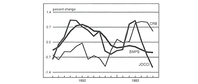
Nevertheless, the run-up in commodity prices and commodity price indexes that occurred between January 1993 and March 1993 (see figure 1) generated significant concerns about inflation. Should we have been concerned? Not really. Commodity prices are among the most sensitive and volatile of existing economic indicators, and this characteristic is both their strength and their weakness. In fact, since commodity prices respond with vigor to a wide variety of economic events, it is a difficult and often treacherous exercise to determine the meaning of any particular surge. Weather-related phenomena, for instance, often affect commodity prices enormously without signaling anything about inflationary pressures.
1. Commodity price indexes

Sources: JOCCI: Center for International Business Cycle Research, Columbia University. CRB: Commodity Research Bureau, Inc. SMPS: U.S. Departments of Commerce and Labor and Commodity Research Bureau, Inc.
In this Chicago Fed Letter we present a new approach to interpreting commodity price changes that allows us to separate price changes that have significant implications for inflation and output growth from price changes that merely reflect the rapidly shifting idiosyncratic circumstances of individual commodity markets. We use this year’s run up as an example of how a superficial interpretation of commodity price changes can be highly misleading.
Our analysis begins with two simple but critical realities. First, at any given moment, not all commodity prices are signaling the same events. Second, each commodity price is signaling something about price and about output at the same time. Once we recognize the importance of these two attributes, we can identify the price signals, analyze their individual content, and then compare and contrast signals in order to understand better the forces behind them.
Commodity price indexes: turning apples and oranges into juice
One way of translating a wide range of individual price signals into common units is by constructing indexes. In simple terms, commodity price indexes are typically calculated as the weighted average of the different component commodity prices. In our analysis, we look at three indexes: the Commodity Research Bureau’s Futures Price Index (CRB) of 21 equally weighted commodities, the Journal of Commerce Industrial Price Index (JOCCI) of 18 components with individual weights, and the Change in Sensitive Materials Prices (SMPS).1 SMPS is calculated as the moving average of the monthly changes in the Index of Sensitive Materials Prices, which itself includes 25 components.
Analysts often use commodity price indexes to construct forecasts of future inflation. A sudden surge in any of these composite indexes may need to be viewed with caution, however, since it may result from a temporary run-up in just one component of the index. An alternative approach to using these indexes to forecast inflation is to construct forecasts based on the prices of single commodities. Typically, each of these individual forecasts is less accurate than a forecast based on the composite index, since the composite index at least allows some of the randomness that affects individual commodity prices to average out. Nevertheless, the overall pattern of the individual commodities’ forecasts can still tell us something about isolated and short-lived price surges.
In our analysis, we produce inflation forecasts both from commodity price indexes—CRB, JOCCI, SMPS—and individual commodity prices, which we call indicators. We measure inflation as the percent change in the level of the Consumer Price Index (CPI) from fourth quarter to fourth quarter, and our forecasts rely on past data of both the CPI and the indicator. Moreover, our results are estimated with data through the first quarter of 1993. This allows us to focus on the run-up in commodity prices that occurred at the beginning of 1993 to show how commodity prices can at times be misleading indicators of future inflation.
Lumber: the effect of an outlier
Lumber underwent a temporary surge in prices during the first three months of 1993. That surge was due to a weather-related drop in lumber production combined with a temporary increase in the demand for building materials. The spot price of lumber reached an unprecedented $439 per thousand board feet in March. By June, the price of lumber had fallen to approximately $236 per thousand board feet, which was close to its late 1992 level. The surge in lumber prices produced a surge in the commodity price indexes, which also rose from January through March. For example, JOCCI went from 98 in January to over 100 in March. Similarly, CRB rose from 201 to 210 over the same period. By June 1993, JOCCI and CRB had fallen back to approximately 96 and 205, respectively.
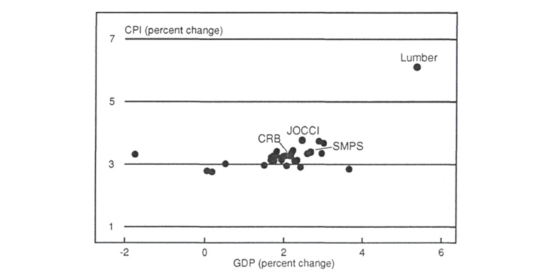
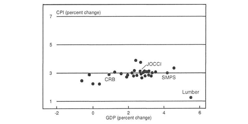
Figure 2 presents inflation forecasts for 1993 and 1994 based on each of the three commodity price indexes and on 28 individual commodity prices.2 Forecasts for 1993 range from a low of 2.76% to a high of 6.12%, with a mean and median of 3.32% and 3.27%, respectively. Lumber produced the highest 1993 inflation forecast, 6.12%. Clearly, the 1993 inflation forecasts from commodity price indexes in figure 2 would have been lower were it not for the temporary surge in lumber prices. The 1994 inflation forecasts, also in figure 2, confirm this point. In fact, they are considerably lower than the 1993 forecasts and range between 1.28% and 3.89%, with a mean and median of 2.91% and 2.96%, respectively. The apparent price pressures displayed in 1993 by some of the indicators clearly disappear in 1994.
2. Inflation forecasts (% change)
| Indicators | 1993 4th quarter |
1994 4th quarter |
|---|---|---|
| JOCCI | 3.78 | 3.14 |
| SMPS | 3.39 | 3.02 |
| CRB | 3.29 | 2.91 |
| Lumber | 6.12 | 1.28 |
| Cocoa beans | 2.97 | 2.72 |
| Burlap | 3.11 | 3.13 |
| Coffee | 3.02 | 2.87 |
| Copper scrap | 3.30 | 3.14 |
| Cotton | 3.74 | 2.85 |
| Eggs | 3.42 | 3.17 |
| Flour | 2.76 | 2.24 |
| Hogs | 3.29 | 3.07 |
| Lead | 3.36 | 2.79 |
| Soybean oil | 3.35 | 2.96 |
| Cottonseed oil | 3.13 | 2.79 |
| Pork bellies | 3.23 | 2.89 |
| Broilers | 3.39 | 2.94 |
| Rubber | 3.12 | 2.66 |
| Steel scrap | 3.68 | 3.00 |
| Silver | 3.28 | 3.03 |
| Steers | 3.45 | 3.08 |
| World sugar | 3.27 | 2.83 |
| Wool | 2.85 | 3.89 |
| Wheat | 2.79 | 2.23 |
| Zinc | 3.15 | 3.35 |
| Gold | 2.96 | 3.08 |
| Plywood | 3.32 | 2.46 |
| Platinum | 3.13 | 3.10 |
| Cotton cloth | 2.91 | 3.76 |
| Fuel oil | 3.26 | 3.02 |
| Copper | 3.22 | 2.80 |
The wide range of inflation forecasts for 1993 shown in figure 2 indicates that because commodity prices vary considerably, forecasts based on the price of a single commodity are not useful by themselves. Moreover, composite indexes may also produce very different forecasts depending on the weight assigned to any one component and on the price variability of that component. It is possible, in fact, that a transient price increase in just one component of the index may cause a commodity price index to send an unwarranted signal of inflationary pressures.
Despite these compositional concerns in interpreting commodity price index movements, it appears that many economists and business analysts react to these temporary run-ups in commodity prices by changing their forecasts of inflation. For example, the Blue Chip Economic Indicators’ forecast of CPI growth for 1993 stood at 3.1% in February, just before the sharp rise in prices.3 After the larger-than-anticipated increases in some commodity prices, the Blue Chip’s consensus forecast of CPI growth for 1993 rose to 3.2% in April and 3.3% in May, suggesting that a number of economists had altered their expectations of inflation in response to the surge in commodity prices. By the time the indexes fell in August 1993, however, the Blue Chip’s consensus forecast for CPI growth in 1993 was back to a little more than 3.1%.
Taking the analysis one step further
To get a clearer assessment of the reliability of the forecasts produced by the indicators in our analysis, we use each indicator in figure 2 to produce forecasts of CPI and real gross domestic product (GDP) growth rates for 1993 and 1994. We consider an indicator reliable if the forecasts it provides for CPI and GDP growth seem reasonable and can be rationalized in the light of other economic conditions. For example, if the price of tea in China produced a CPI forecast of 5% and a GDP forecast of -20%, that would be difficult to rationalize in the absence of a large, identifiable supply shock to the U.S. economy. The two forecasts could thus be rationalized but would not seem reasonable given the current state of the U.S. economy. Using this approach, we can filter out indicators that seem subject to idiosyncratic abnormalities.
We plot the indicators’ forecasts of CPI and GDP growth (fourth quarter over fourth quarter) in figures 3 and 4. The horizontal axis measures each indicator’s GDP growth forecast; indicators that predict rapid growth in GDP tend toward the right-hand side, slow growth toward the left. The vertical axis measures each indicator’s CPI growth forecast; indicators that predict high inflation tend toward the top, low inflation toward the bottom.
3. 1993 forecasts from commodity-based indicators

4. 1994 forecasts from commodity-based indicators

Figure 3 shows just how aberrant lumber’s 1993 inflation forecast is. Most of the other forecasts in the figure tend to group between 2.97% and 3.74%. Viewed in this context, lumber’s 6.12% seems more than a little odd. Of course, an inflation rate of over 6% in 1993 might not seem so unlikely if one believed that real activity was going to grow 5% in 1993, which is lumber’s forecast for GDP growth. Lumber was not just signaling previously undetected inflation, it was also forecasting a massive undetected surge in economic activity. Clearly, lumber’s forecasts can be rationalized, but they do not seem reasonable. It is important, therefore, to analyze a forecast based on an individual commodity price not only in the context of other such forecasts, but also in the context of whatever else that commodity price is forecasting. A two-part reality check such as this can help one assess the reasonableness of other forecasts based on single commodity prices.
Unpredictable price movements such as those in lumber are not one-time events. Between March and June 1993, when lumber prices fell almost 50%, the spot price of gold jumped over 12%. It continued to rise to a peak of over $400 per ounce during the week of August 4, then declined rapidly. This surge in gold prices generated another distortion in the commodity indexes, which without detailed analysis might have seemed like a continuation of the earlier warning based on lumber prices.
There is still another reason to believe that price increases during the first half of 1993 in commodities such as lumber and gold were only temporary surges due to a variety of short-lived economic events. As figure 4 shows, anomalous inflation forecasts clearly disappear in 1994, and the “cloud” of forecasts from commodity prices and commodity price indexes moves toward the lower portion of the graph, indicating lower overall inflation forecasts.
Conclusion
The above analysis points out that forecasts from economic indicators can be distorted by a large variety of events, and that the simple use of any single indicator can be misleading. No amount of statistical analysis can deal with the incredible variety of special factors that can distort any specific model. But breaking those predictions apart can often yield valuable qualitative information.
Tracking Midwest manufacturing activity
Manufacturing output index (1987=100)
| Aug. | Month ago | Year ago | |
|---|---|---|---|
| MMI | 119.9 | 119.5 | 112.5 |
| IP | 111.8 | 111.5 | 106.9 |
Motor vehicle production (millions, saar)
| Aug. | Month ago | Year ago | |
|---|---|---|---|
| Cars | 5.0 | 5.4 | 5.4 |
| Light trucks | 4.3 | 4.0 | 3.7 |
Purchasing Managers’ Surveys: production index
| Sept. | Month ago | Year ago | |
|---|---|---|---|
| MW | 67.5 | 56.3 | 58.4 |
| U.S. | 53.5 | 51.6 | 52.6 |
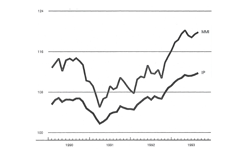
Manufacturing output index, 1987=100

The Midwest Manufacturing Index (MMI) depicted a modest increase in industrial output in August. After the surge in output in late 1992 and early 1993, there was a clear loss of momentum during the summer. Within the overall MMI, a number of important Midwest industries experienced slower growth or actual declines in the summer, most notably the motor vehicle sector.
Industry assembly data during June, July, and August echoed the erosion in the motor vehicle component of the MMI, but much of this decline can be attributed to factors other than slowing demand. Auto dealers’ share of total retail sales has continued to rise in recent months and has helped shore up expectations for expansion in Midwest manufacturing activity during the balance of 1993. Purchasing managers’ surveys showed renewed vigor in September.
Notes
1 The Commodity Research Bureau’s Future Price Index (1967=100) is compiled by the Commodity Research Bureau, Inc., Chicago. The Journal of Commerce Industrial Price Index (1980=100) is compiled by the Center for International Business Cycle Research at Columbia University, New York. The Change in Sensitive Material Prices (1982=100) is compiled by the U.S. Department of Commerce, U.S. Department of Labor, and Commodity Research Bureau, Inc..
2 Commodity prices are averages of spot prices from the Wall Street Journal.
3 The data are from Blue Chip Economic Indicators, Capitol Publications Inc., Alexandria, VA, February-August 1993. The Blue Chip Economic Indicators’ consensus forecast is the average forecast from a survey of 51 economists. In this Chicago Fed Letter, we quote the Blue Chip’s inflation forecasts on a fourth quarter over fourth quarter basis. We calculated them as the average of the Blue Chip’s consensus forecasts of the CPI quarterly percent changes at annual rates.


